39
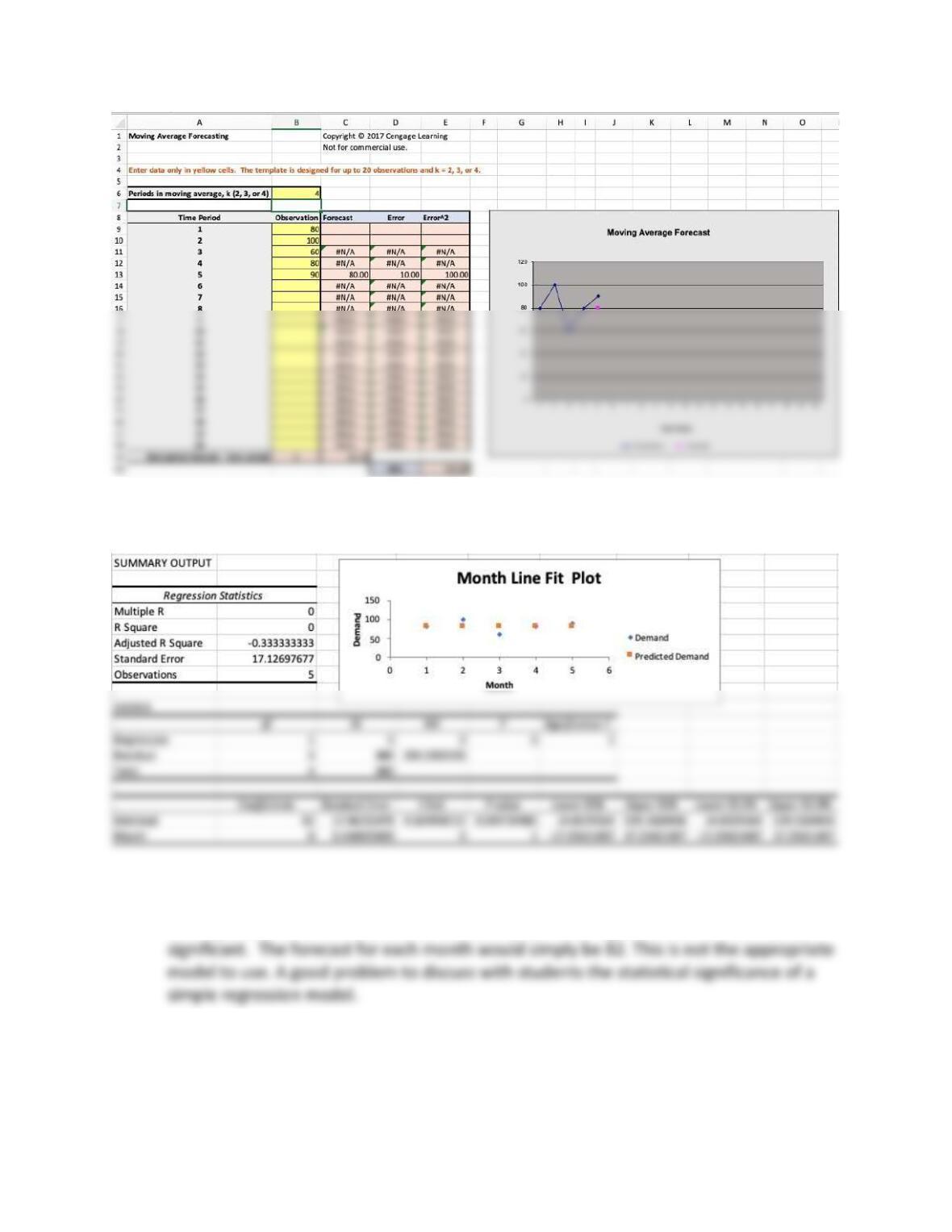
b. Develop a linear regression model using Excel and compute a forecast for June, July,
and August.
c. Compare these results and explain the implications of the regression model.
The regression trend line is flat with a slope of 0, so the regression is not statistically
46. The president of a small manufacturing firm is concerned about the continual growth in
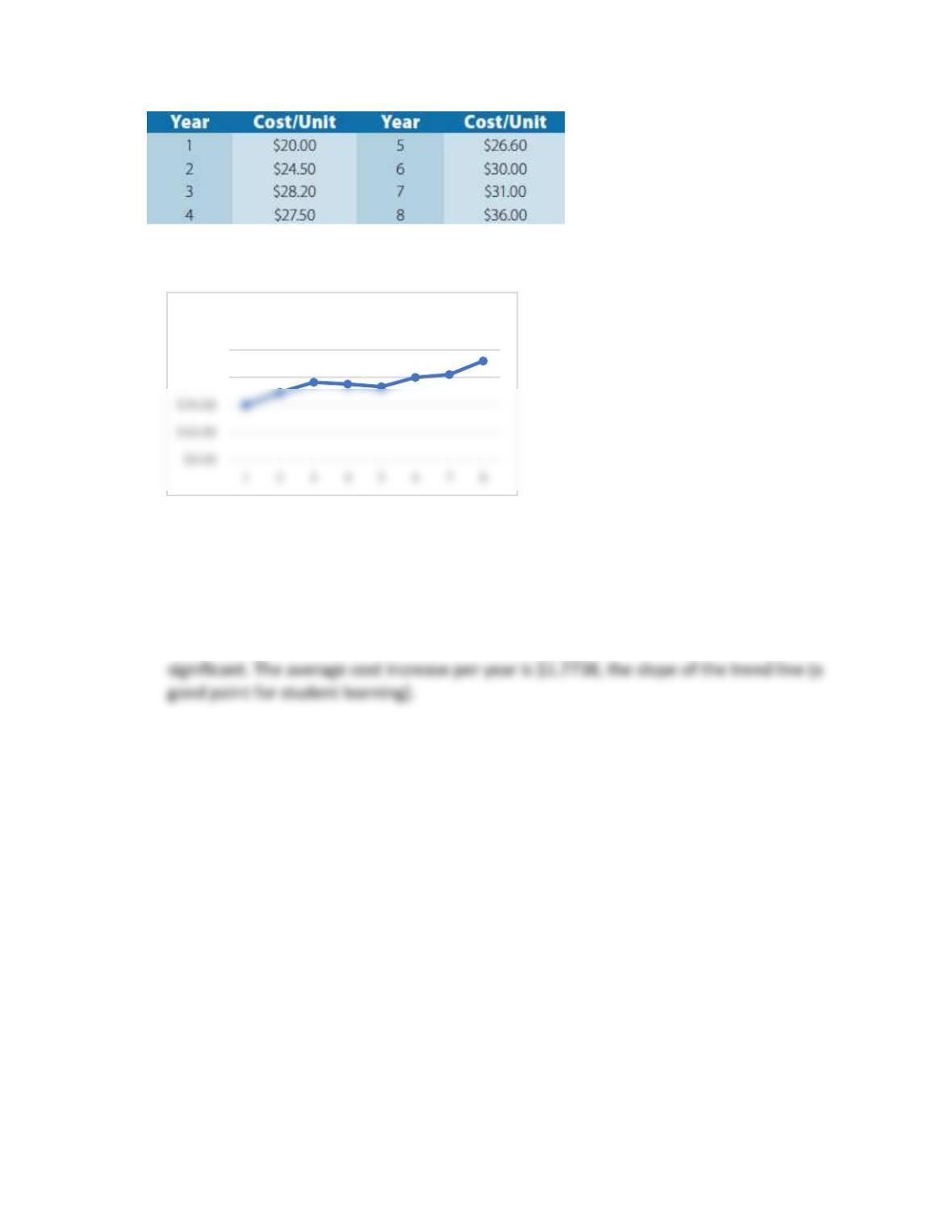
manufacturing costs in the past several years. The data series of the cost per unit for the
firm’s leading product over the past eight years are given as follows:
40
a. Plot this time series on a spreadsheet. Does a linear trend appear to exist?
The data appear to have a linear trend.
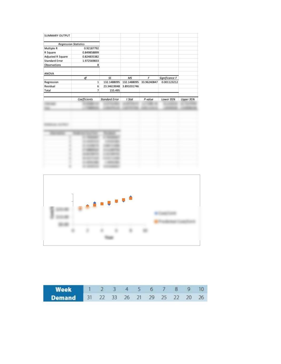
b. Use Excel to develop a simple linear regression model for these data. What average cost
increase has the firm been realizing per year?
The trend line is Unit Cost = 19.993 + 1.7738 Year. R-square = 0.849 and the model is
$30.00
$40.00
Cost/Unit
41
47. A chain of grocery stores had the following weekly demand (cases) for a particular brand of
laundry soap.
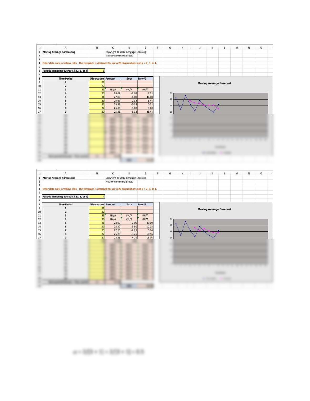
a. Use the Moving Average Excel template to develop three- and four-period moving
average forecasts, and compute MSE for each. Which provides the better forecast?
What would be your forecast for week 11?
$30.00
$40.00
Year Line Fit Plot
42
Based on these results, the 3-month model has a lower MSE = 14.22. The forecast for week
11 would be 22.67. The MSE for a 4-period moving average is 16.49 and a forecast for
week 11 of 23.25.
b. Use the Exponential Smoothing Excel template to develop an exponential-smoothing
forecast using the alpha smoothing constant value determined by Equation 9.6.
43
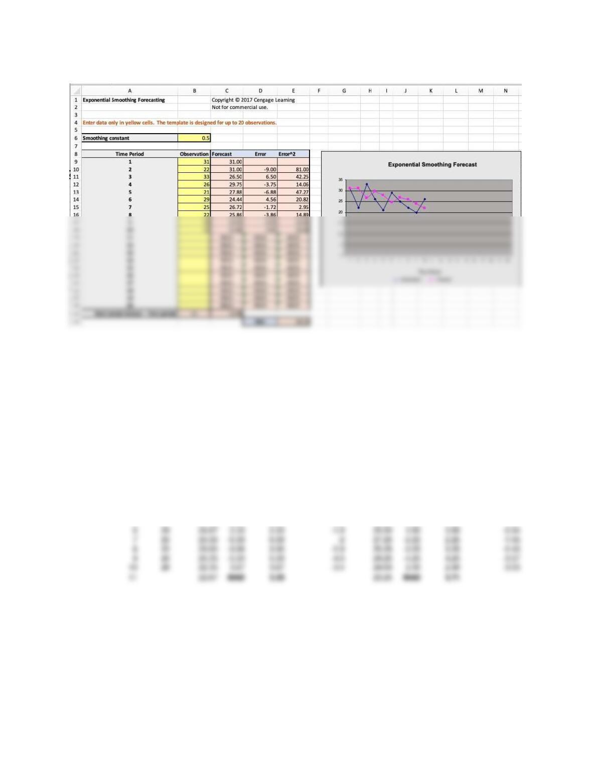
MSE = 28.33 for
= 0.5 and MSE = 26.83 for
= 0.4. You might want to point out to
students that Equation 9.6 is simply an approximation for alpha based on k. Still the 3–
month moving average with an MSE = 14.22 is the best model.
c. Compute the tracking signal for a three- and four-period moving average model on a
spreadsheet. Is there any evidence of bias?
Students must build this Excel model and use Equation 9.8.
The tracking signals suggest that the model is generally adequate since it is between
plus/minus 4. An example computation is -7.00/3.71 = -1.89 for the 4-period moving
average.
48. Two experienced managers are resisting the introduction of a computerized exponential
smoothing system, claiming that their judgmental forecasts are much better than any
computer could do. Their past record of predictions is as follows:
Week Sales 3-Month MA Error Abs Error Tracking Signal 4-Month MA Error Abs Error Tracking Signal
131
222
333
426 28.67 -2.67 2.67 -0.8
521 27.00 -6.00 6.00 -2.6 28.00 -7.00 7.00 -1.89
44
These data are available in the Excel worksheet C9 Excel P48 in MindTap.
Compare the manager’s judgmental forecasts to those obtained using time series models.
Are the manager’s judgmental forecasts performing satisfactorily? (Use appropriate Excel
templates and compute error metrics for the manager’s forecasts on a spreadsheet.)
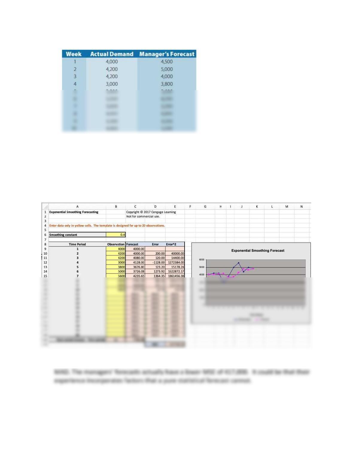
After finding the best value exponential smoothing model with alpha = 0.4, MSE = 567,781.
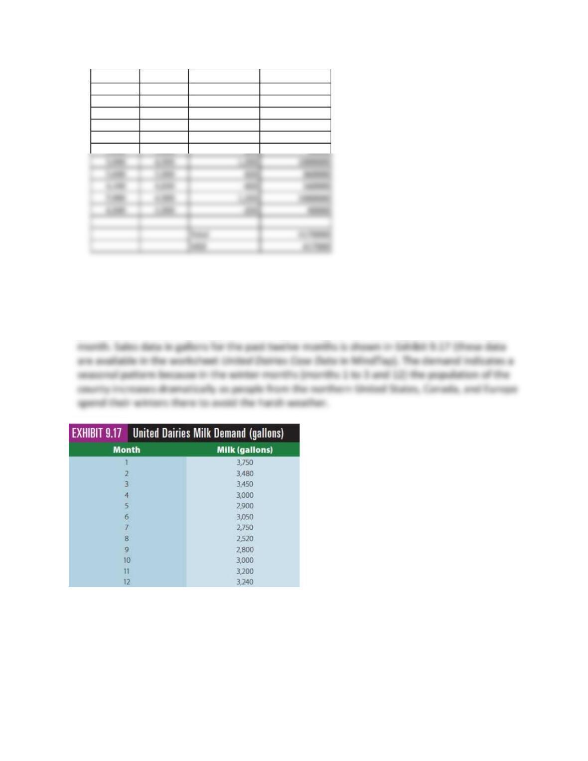
Using Equation 9.1 and building an Excel model to compute MSE for the manager’s
forecast, we find it to be 417,000. Students may use other measurements of error such as
45
Actual Manager (At – Ft)
(At – Ft)2
Demand Forecast
4,000 4,500 -500 250000
4,200 5,000 -800 640000
4,200 4,000 200 40000
3,000 3,800 -800 640000
Teaching Note: United Dairies, Inc. Case Study
United Dairies, Inc. supplies milk to independent grocers in Collier County, Florida. Milk is
perishable so forecast accuracy is critical in predicting the number of gallons of milk sold per
Case Questions for Discussion:
1. What moving average or exponential smoothing model would you recommend to
forecast demand? Clearly show your results and explain your conclusions.
46
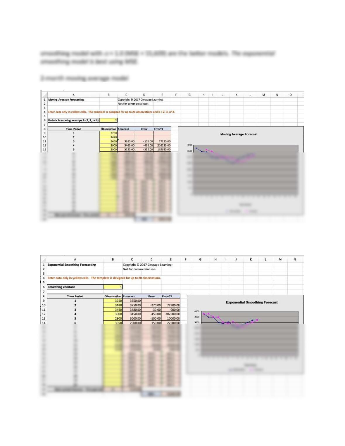
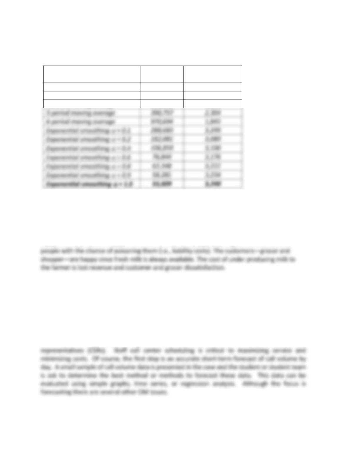
Given the analysis here, the 2-period moving average (MSE = 80,653) and the exponential
Exponential Smoothing with Alpha = 1.0
47
Summary:
Forecasting Method
MSE
Forecast for
Month 13(gallons)
2-period moving average
80,653
3,220
3-period moving average
113,494
3,147
4-period moving average
118,352
3,060
5-period moving average
390,757
2,304
6-period moving average
970,694
1,845
Exponential smoothing
Exponential smoothing
Exponential smoothing
Exponential smoothing
Exponential smoothing
2. What might the economic impact be of over or under forecasting here for this perishable
commodity?
The cost of over producing milk to the farmer (supplier) is using excess labor, energy, and
equipment to produce milk, part of which is throw away (spoiled) or given to charities and
Teaching Note: BankUSA: Forecasting Help Desk Demand by Day Case Study
Overview
The case describes a telephone call center (contact center) where 98% of the call volume is
internal customers (i.e., the bank’s sales force, trust administrators, branch managers, wealth
advisors, etc.). Accurate and quick answers are expected from the customer service

48
Case Questions for Discussion:
1. What are the service management characteristics of the CSR job?
This is an important question and we find that students do not fully appreciate the magnitude of
“service management jobs” unless you carefully discuss it in class. Discuss each component –
technical and operational skills, human interaction skills, and face–to–face marketing and cross–
2. Define the mission statement and strategy of the Help Desk contact center? Why is the
Help desk important? Who are its customers?
The Help Desk’s mission is “to provide accurate and timely resolution of customer problems and
3. How would you handle the customer affected by the inaccurate stock price in the banks
trust account system? Passive or proactive approach? Justify your answer.
49
Two options exist as follows: (1) If the stock price is in error correct this customers account
statement, call them and apologize, and immediately mail a corrected account statement.
4. Using the data on Call Volume in the table, how would you forecast short-term demand?
Moving Average (k) MSE
2 5,058
3 5,177
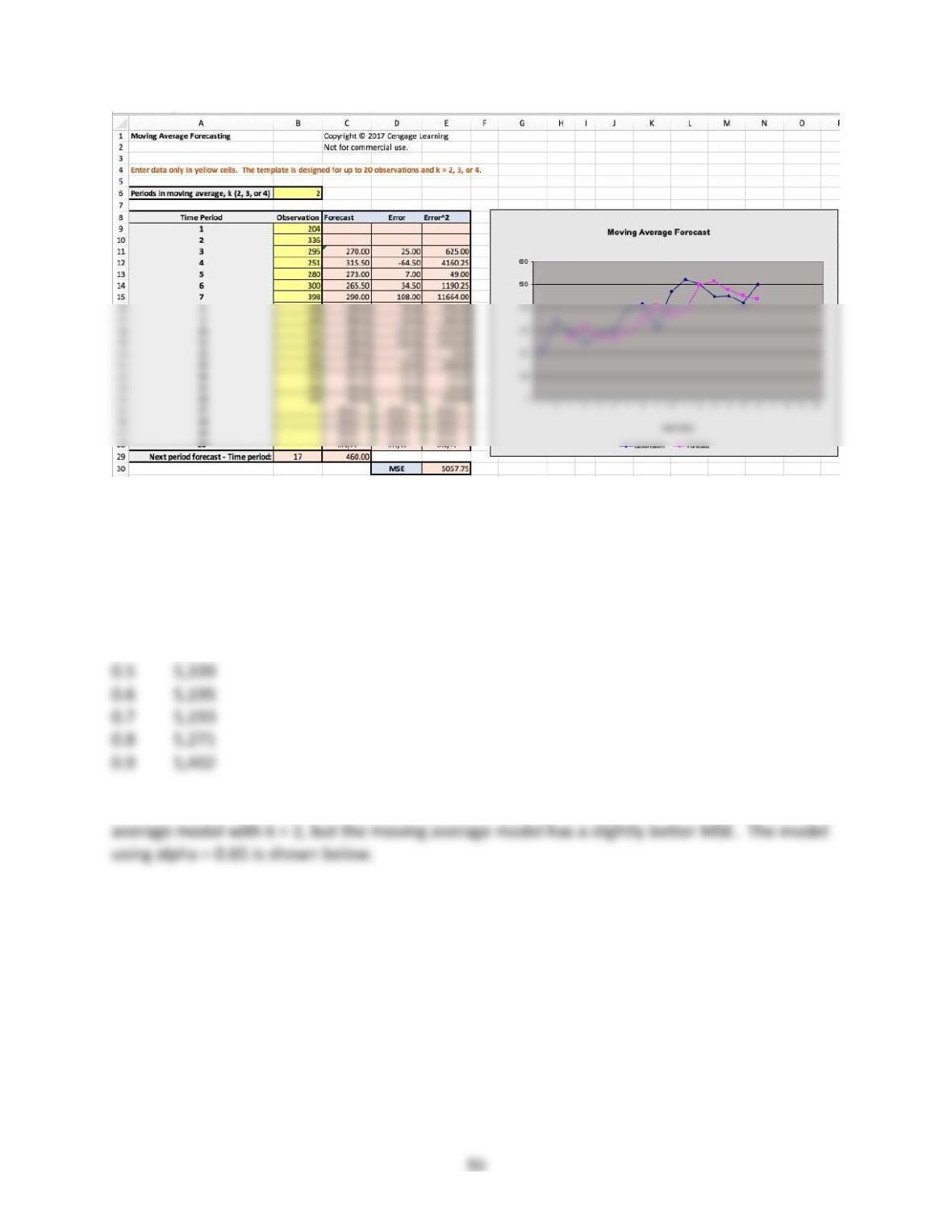
Using the exponential smoothing template, we find:
Alpha MSE
0.1 16,947
0.2 9,410
0.3 6,798
0.4 5,761
The exponential smoothing model with alpha = 0.6 or 0.7 provides similar results as the moving
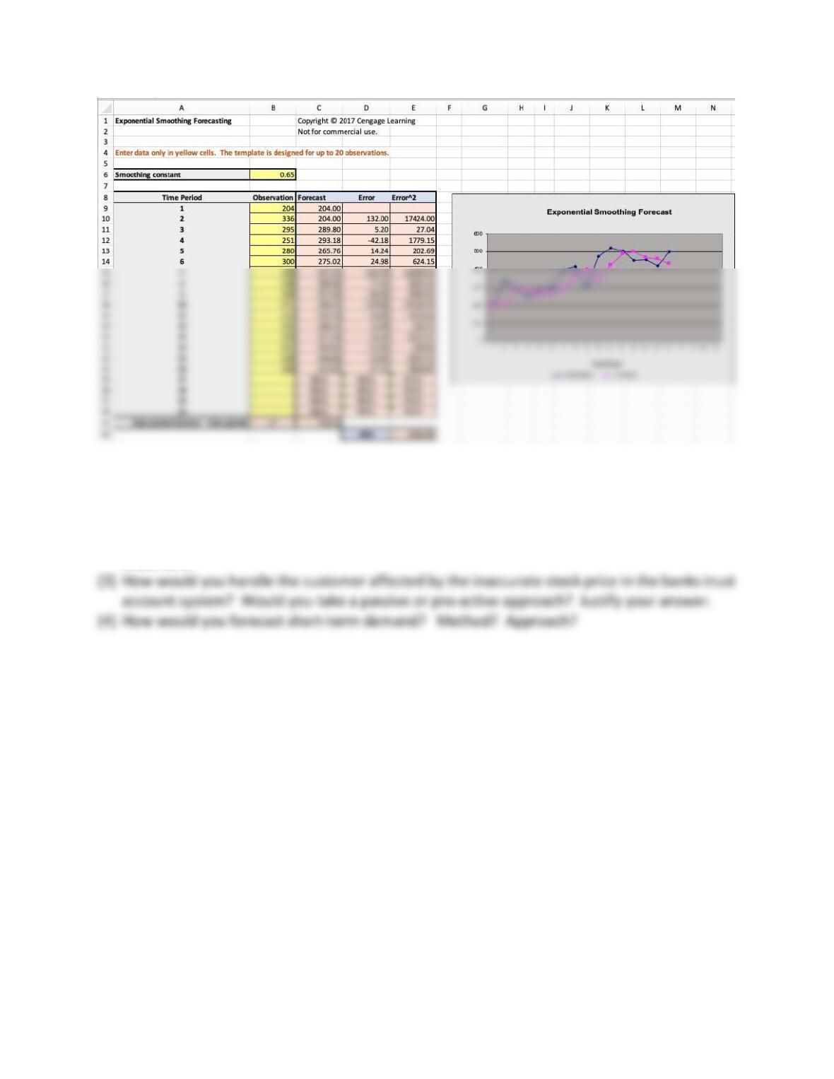
51
Teaching Plan
(1) What are the service management characteristics of the CSRs job?
(2) Define the mission statement and strategy of the Help Desk? Why is the Help desk
INTEGRATIVE CASE: HUDSON JEWELERS
A complete teaching note for all chapters is available in the Instructor Resources online.
Instructors should read the entire case and most of the case assignments at the end of each
chapter. Then decide if you want to assign all or part of the case questions.
Chapter 9 Case Question for Discussion:
1. The worksheet Hudson Demand Case Data in MindTap provides the number of visits over
one year from January to December (52 weeks). Chart the data in Excel and explain the
characteristics of the time series. How would you forecast future demand for customer
visits? What criteria will you use to determine a “good” forecast? What methods would
you use, and why? What is your final recommendation with respect to a forecasting
method?
52
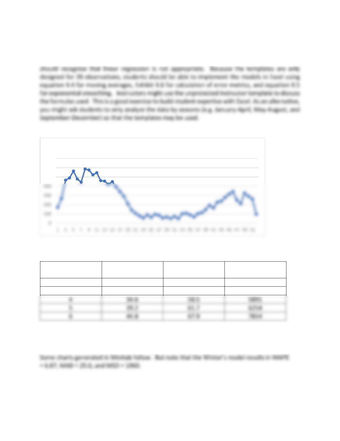
A chart of weekly visits is shown below. The data are highly seasonal. While more advanced
techniques for time series with seasonality might be used, such as Winter’s model, we only
expect students to use the basic moving average and exponential smoothing models. They
Hudson Jewelers Moving Average Results
Moving Average
Length
MAPE
MAD
MSD
2
28.2
54.3
5012
3
31.4
56.2
5270
4
34.6
58.5
5891
5
39.2
61.7
6254
6
44.8
67.9
7814
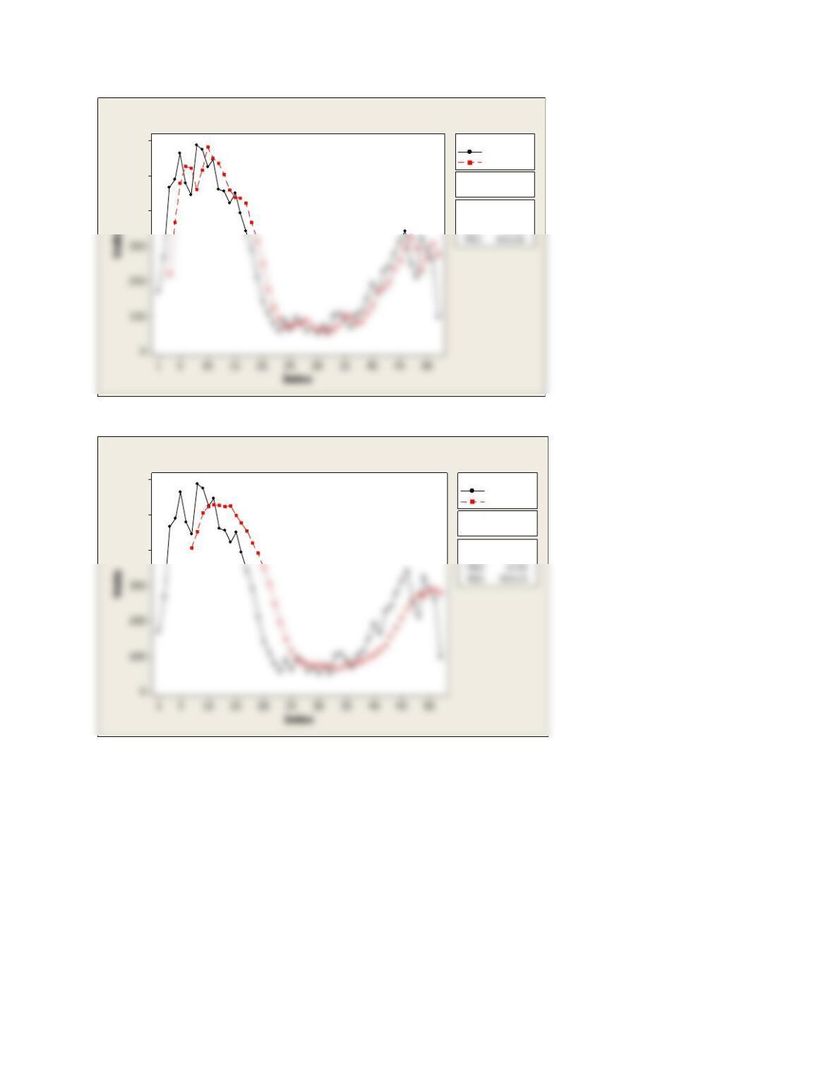
The moving average results indicate with k = 2 weeks we minimize MAPE, MAD, and MSD.
Winter’s model is more appropriate for cyclical variation, but beyond the scope of this text.
500
600
700
Weekly Visits
53
600
500
400
Length 2
Moving Average
MAPE 28.16
Accuracy Measures
Actual
Fits
Variable
Moving Average Plot for Visits
600
500
400
Length 6
Moving Average
MAPE 44.85
Accuracy Measures
Actual
Fits
Variable
Moving Average Plot for Visits
54
600
500
400
Alpha 1.13881
Smoothing Constant
MAPE 25.09
Accuracy Measures
Actual
Fits
Variable
Smoothing Plot for Visits
Single Exponential Method
Advanced Models
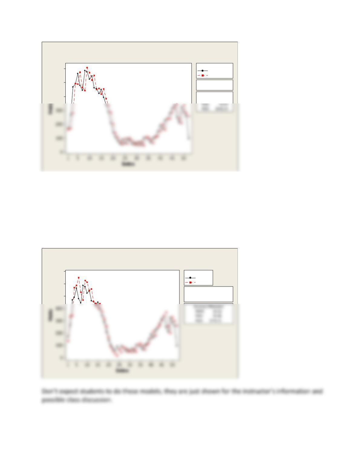
We show you more advanced models for-your-information but we do not expect undergraduates
to do these advanced models. Some MBAs may be capable of doing the more advanced models.
But with this difficult highly seasonal demand pattern it is best for you to see some of the more
advanced models.
700
600
500
Alpha (level) 0.921605
Gamma (trend) 0.283053
Smoothing Constants
Actual
Fits
Variable
Smoothing Plot for Visits
Double Exponential Method
55
Polynomial Regression
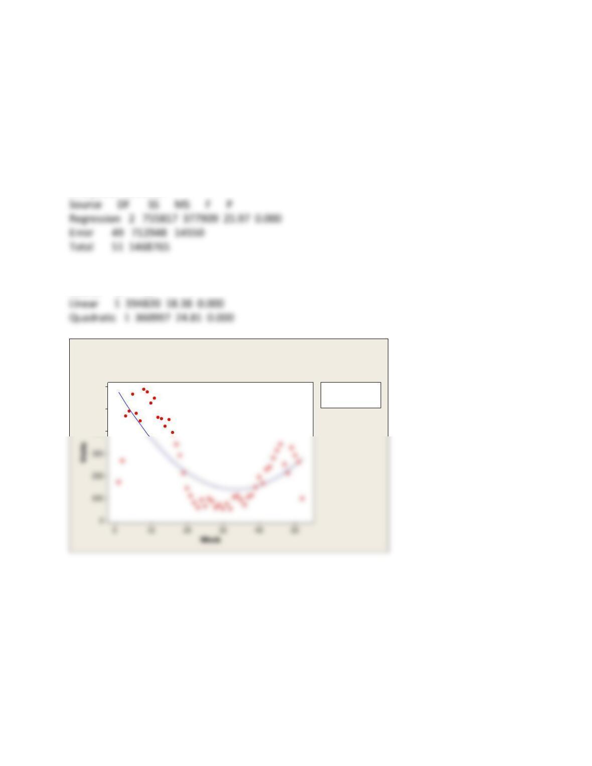
The regression equation is
Visits = 603.2 – 27.74 Week + 0.4138 Week**2
S = 120.623 R-Sq = 51.5% R-Sq(adj) = 49.5%
Analysis of Variance
Sequential Analysis of Variance
Source DF SS F P
600
500
400
S 120.623
R-Sq 51.5%
R-Sq(adj) 49.5%
Fitted Line Plot
Visits = 603.2 – 27.74 Week
+ 0.4138 Week**2
56
600
500
400
Alpha (level) 0.2
Gamma (trend) 0.2
Delta (seasonal) 0.2
Smoothing Constants
Actual
Fits
Variable
Winters’ Method Plot for Visits
Multiplicative Method
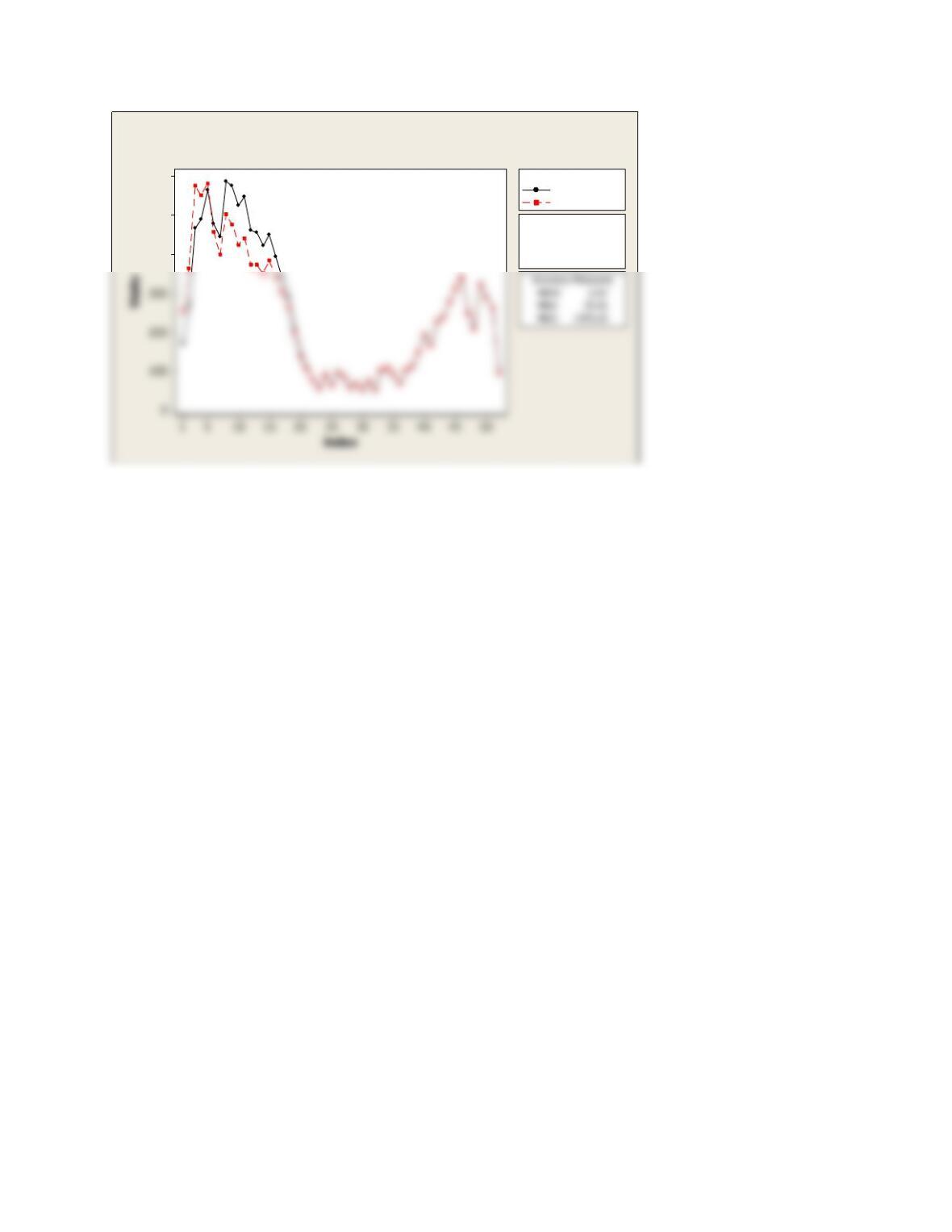
Winter’s model works very well and better (lower MAD, MSE, and MAPE%) than a 2-period moving
average over 52-weeks.