9 – 1
Chapter 9
Linear Programming Applications
Learning Objectives
1. Learn about applications of linear programming that have been encountered in practice.
2. Develop an appreciation for the diversity of problems that can be modeled as linear programs.
Note to Instructor
The application problems of Chapter 9 have been designed to give the student an understanding and
appreciation of the broad range of problems that can be approached by linear programming. While the
problems are indicative of the many linear programming applications, they have been kept relatively small in
Chapter 9
9 – 2
Solutions:
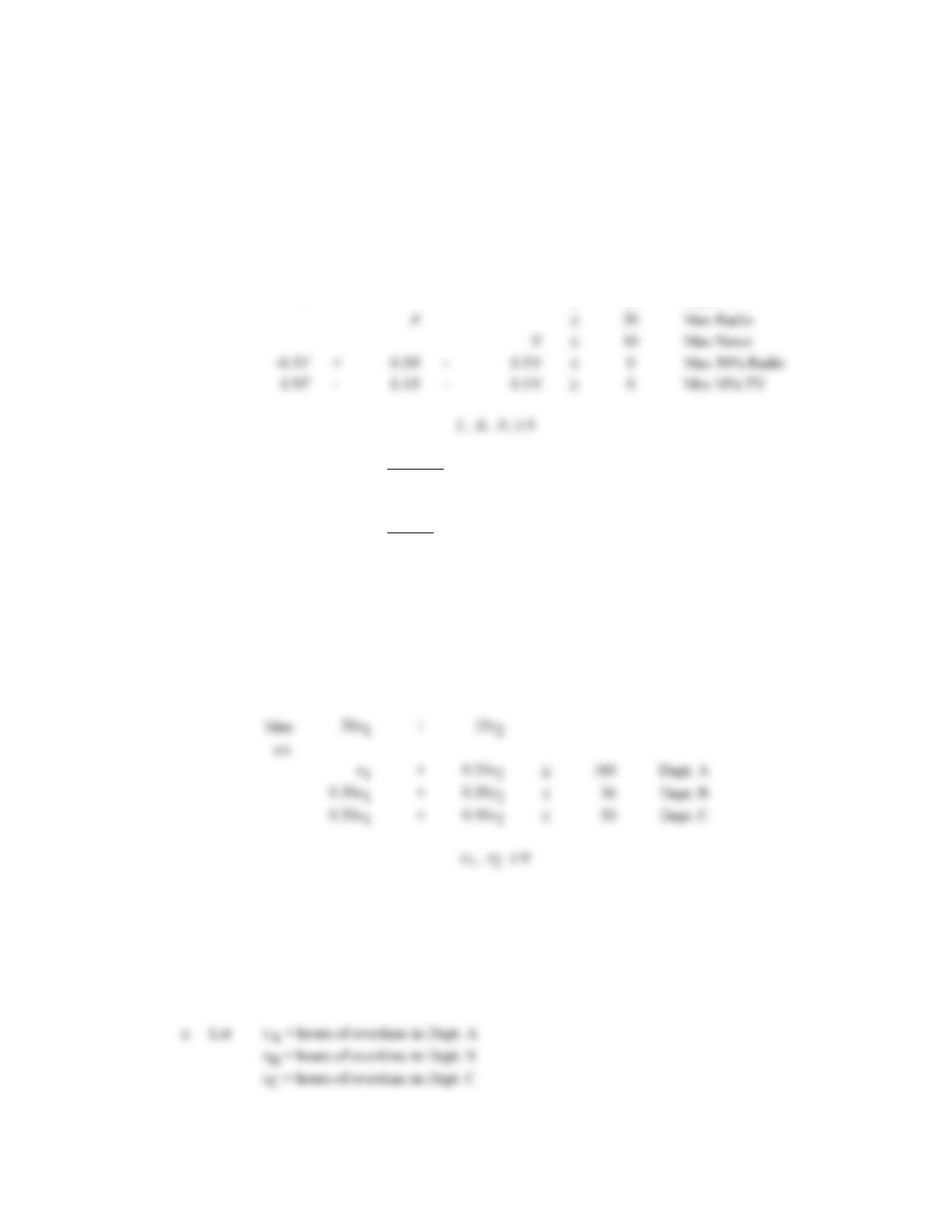
1. a. Let T = number of television spot advertisements
R = number of radio advertisements
N = number of newspaper advertisements
Max
100,000T
+
18,000R
+
40,000N
s.t.
2,000T
+
300R
+
600N
18,200
Budget
20
Max Radio
N
10
Max News
+
–
Max 50% Radio
–
–
Min 10% TV
T
10
Max TV
Budget $
Solution:
T = 4
$8,000
R = 14
4,200
N = 10
6,000
$18,200
Audience = 1,052,000.
b. The shadow price for the budget constraint is 51.30 and the change of 100 is within the range for
which the shadow price holds. Thus, a $100 increase in budget should provide an increase in
audience coverage of approximately 5,130.
2. a. Let x1 = units of product 1 produced
x2 = units of product 2 produced
Solution: x1 = 77.89, x2 = 63.16, Profit = 3284.21
b. The shadow price for Dept. A is $15.79, for Dept. B it is $47.37, and for Dept. C it is $0.00.
Therefore we would attempt to schedule overtime in Departments A and B. Assuming the current
labor available is a sunk cost, we should be willing to pay up to $15.79 per hour in Department A
and up to $47.37 in Department B.
9 – 3
Max
30x1
+
15x2
–
18xA
–
22.5xB
–
12xC
s.t.
x1
+
0.35x2
–
xA
100
0.30x1
+
0.20x2
–
xB
36
0.20x1
+
0.50x2
–
xC
50
xA
xB
xC
Profit = $3341.34
Overtime
Dept. A
10 hrs.
Dept. B
3.186 hrs
Dept. C
0 hours
Increase in Profit from overtime = $3341.34 – 3284.21 = $57.13
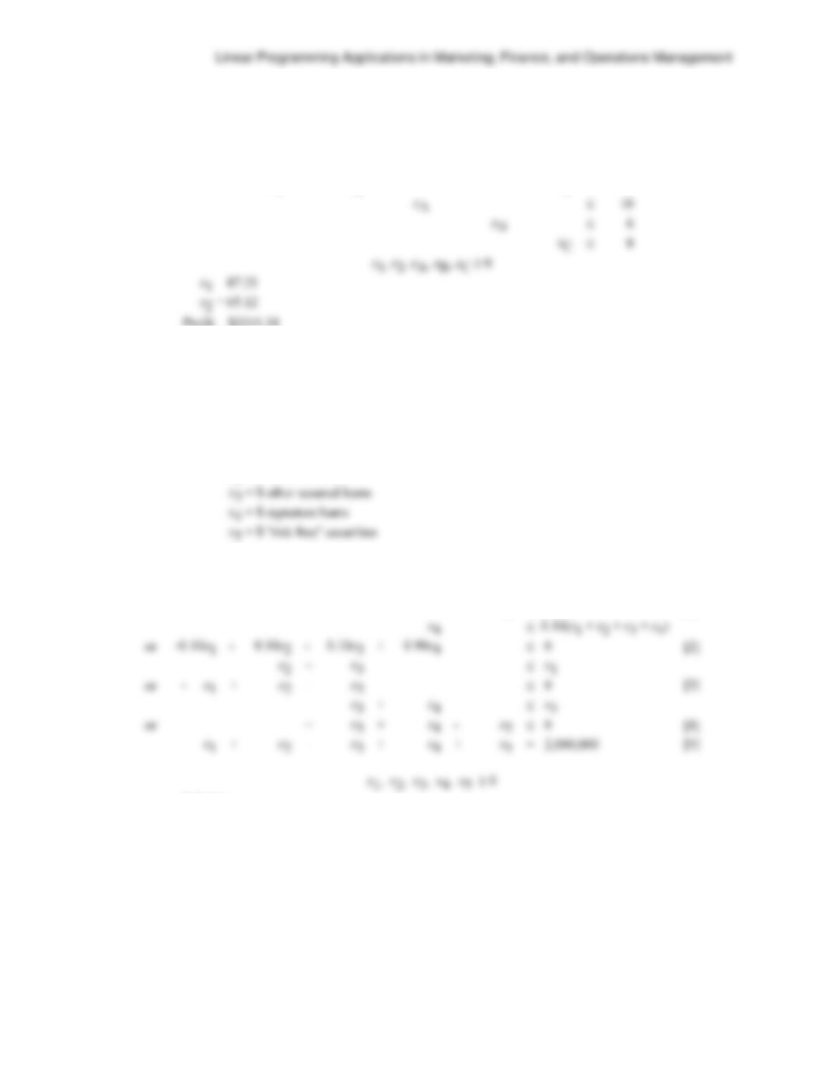
3. x1 = $ automobile loans
x2 = $ furniture loans
Max
0.08x1
+
0.10x2
+
0.11x3
+
0.12x4
+
0.09x5
s.t.
x5
600,000
[1]
–
0.10x2
–
0.10x3
+
0.90x4
[2]
+
x3
– x1
+
+
x3
[3]
x3
+
+
x3
+
–
x5
0
[4]
x1
+
+
x3
+
+
x5
=
[5]
Solution:
Automobile Loans
(x1)
=
$630,000
Furniture Loans
(x2)
=
$170,000
Other Secured Loans
(x3)
=
$460,000
Signature Loans
(x4)
=
$140,000
Risk Free Loans
(x5)
=
$600,000
Annual Return $188,800 (9.44%)
Chapter 9
9 – 4
4.
Let X1 = the number of pounds of Party Nuts to produce
X2 = the number of pounds of Mixed Nuts to produce
X3 = the number of pounds of Premium Nuts to produce
The optimal solution is:
133 1/3 pounds of Party Nuts (or 266 2/3 bags)
666 2/3 pounds of Mixed Nuts (or 1333 1/3 bags)
33 1/3 pounds of Premium Nuts (or 66 2/3 bags)
Profit of $537.33
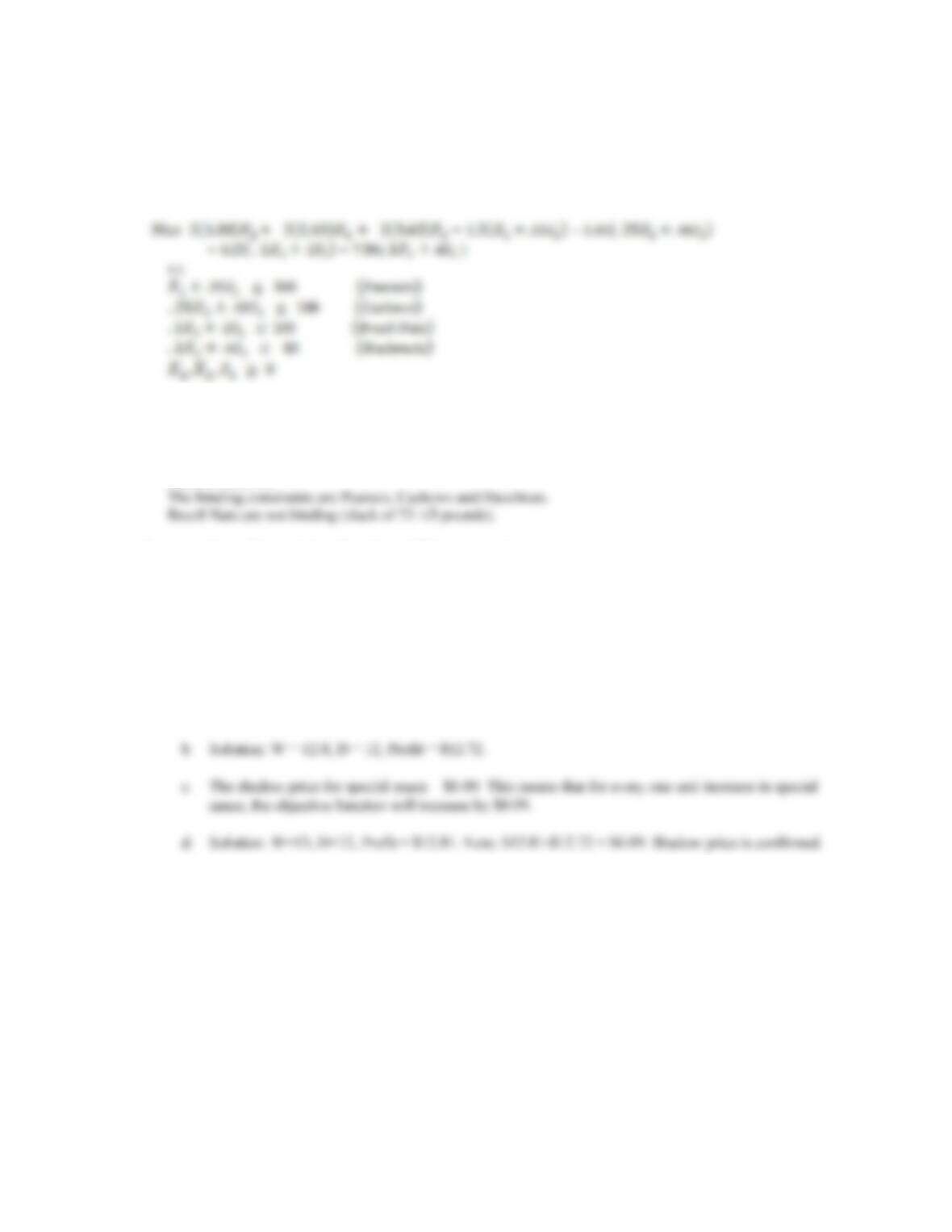
5. a. Let W = number of servings of Wimpy to make
D = number of servings of Dial 911 to make
Max .45 W + .58 D
s.t.
.25 W + .25 D ≤ 20 (Beef)
.25 W + .4 D ≤ 15 (Onions)
5 W + 2 D ≤ 88 (Special Sauce)
5 D ≤ 60 (Hot Sauce)
W, D ≥ 0
6. Let x1 = units of product 1
x2 = units of product 2
b1 = labor-hours Dept. A
b2 = labor-hours Dept. B
Linear Programming Applications in Marketing, Finance, and Operations Management
9 – 5
Max
25x1
+
20x2
+
0b1
+
0b2
s.t.
12x1
+
10x2
–
1b2
=
1b1
+
1b2
6x1
+
8x2
–
1b1
=
0
7. a. Let F = total funds required to meet the six years of payments
G1 = units of government security 1
G2 = units of government security 2
Si = investment in savings at the beginning of year i
Note: All decision variables are expressed in thousands of dollars
Min F
S.T.
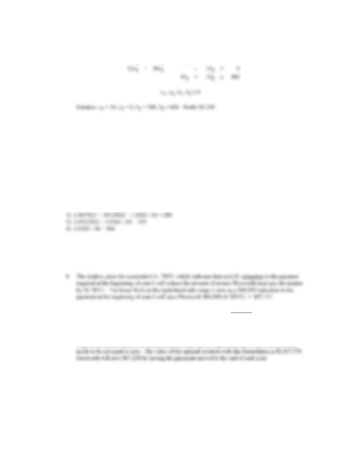
1) F – 1.055G1 – 1.000G2 – S1 = 190
2) .0675G1 + .05125G2 +1.04S1 – S2 = 215
3) .0675G1 + .05125G2 + 1.04S2 – S3 = 240
The current investment required is $1,484,967. This calls for investing $232,394 in government
security 1 and $720,388 in government security 2. The amounts, placed in savings are $329,404,
$180,186 and $442,308 for years 1, 2, and 5 respectively. No funds are placed in savings for years
3, 4, and 6.
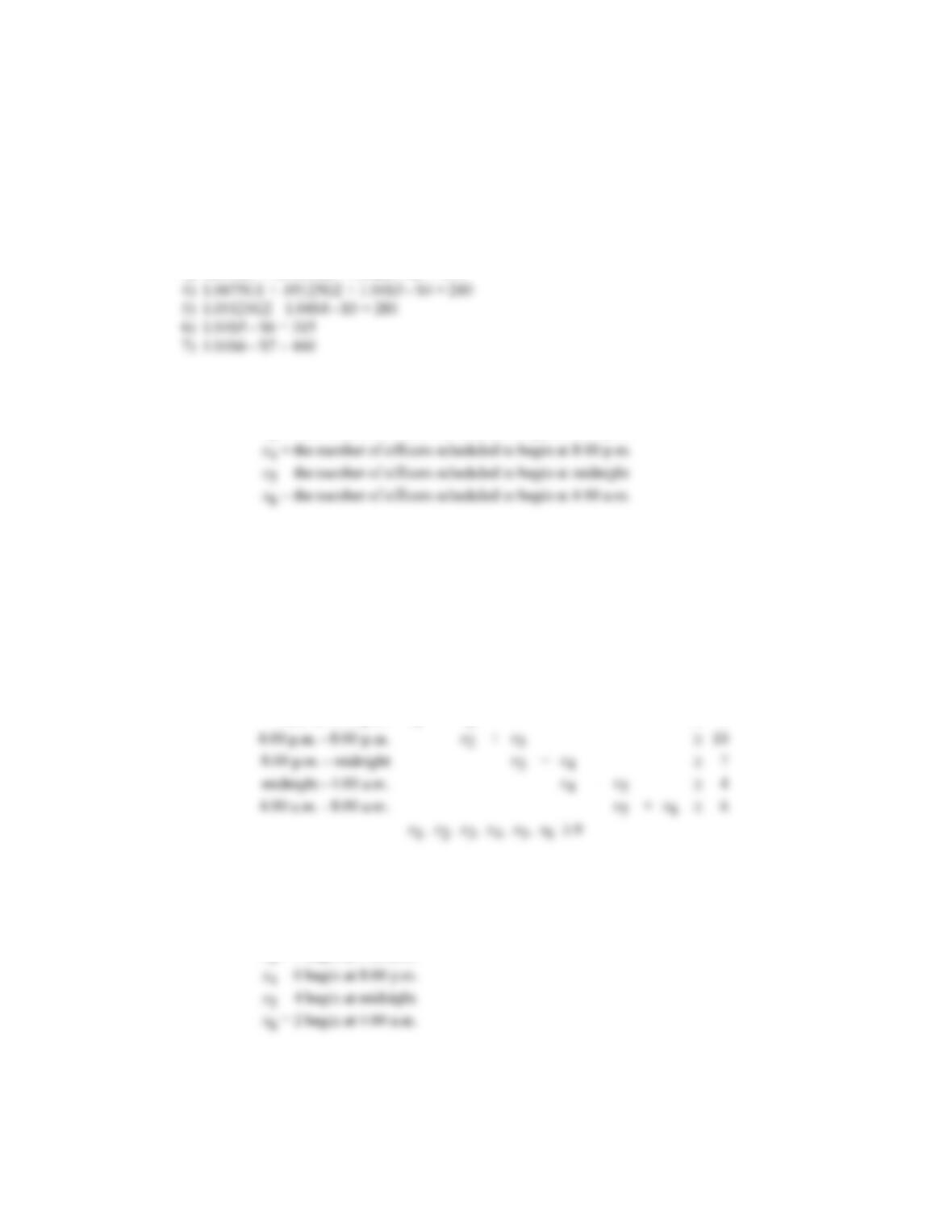
c. The shadow price for constraint 1 is 1.00 shows that every dollar of reduction in the initial payment
is worth $1.00 to Hoxworth (reduces the total needed by $1). So Hoxworth should be willing to pay
anything less than $40,000.
d. To reformulate this problem, one additional variable needs to be added, the right-hand sides for the
Chapter 9
9 – 6
The revised formulation is shown below:
MIN F
S.T.
1) F – 1.055G1 – 1.000G2 – S1 = 0
2) .0675G1 + .05125G2 + 1.04S1 – S2 = 190
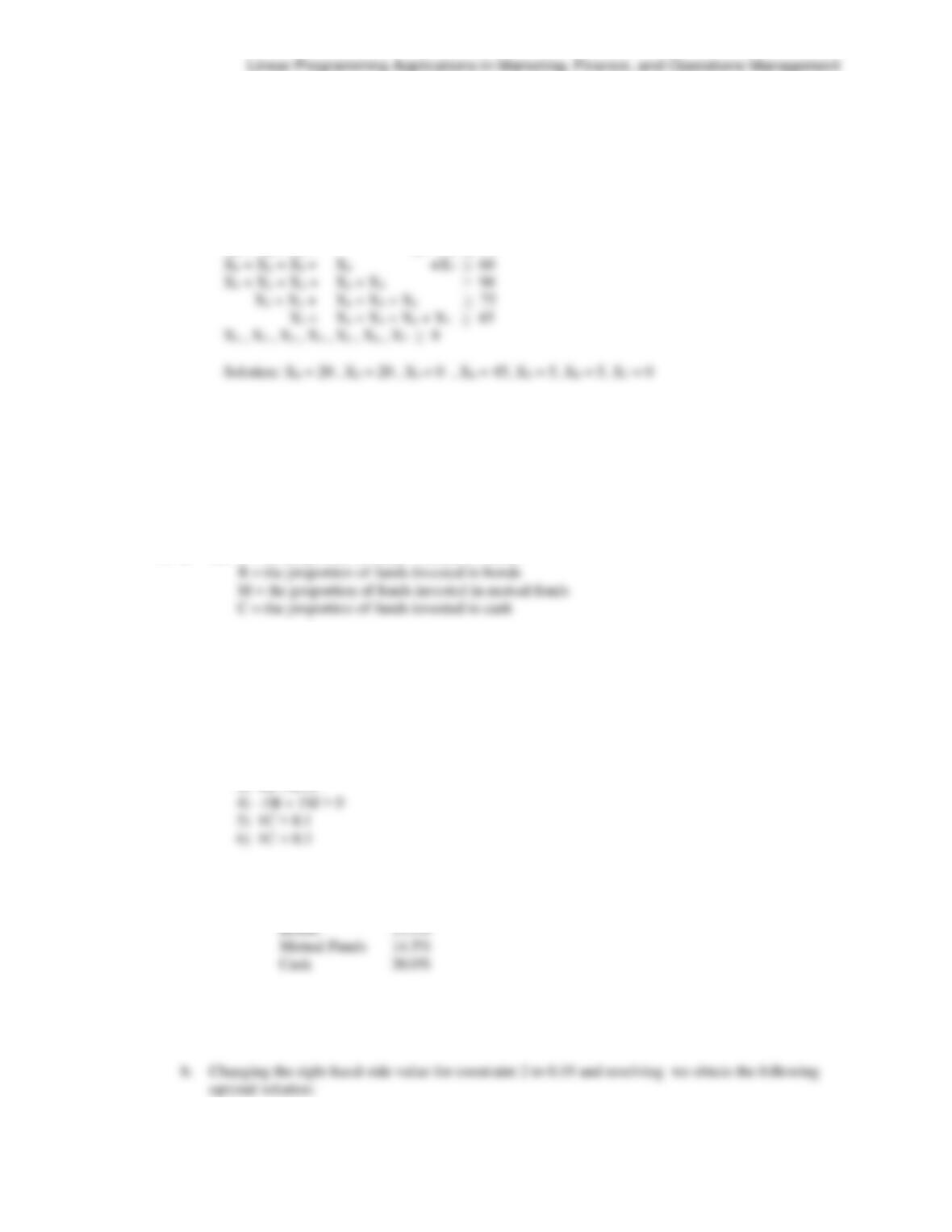
8. Let x1 = the number of officers scheduled to begin at 8:00 a.m.
x2 = the number of officers scheduled to begin at noon
x3 = the number of officers scheduled to begin at 4:00 p.m.
The objective function to minimize the number of officers required is as follows:
Min x1 + x2 + x3 + x4 + x5 + x6
The constraints require the total number of officers of duty each of the six four-hour periods to be at
least equal to the minimum officer requirements. The constraints for the six four-hour periods are as
follows:
Time of Day
8:00 a.m. – noon
x1
+
x6
5
noon to 4:00 p.m.
x1
+
x2
x2
x3
x3
+
x4
7
x4
+
x5
4
x5
+
x6
6
6
Schedule 19 officers as follows:
x1 = 3 begin at 8:00 a.m.
x2 = 3 begin at noon
x3 = 7 begin at 4:00 p.m.
9 – 7
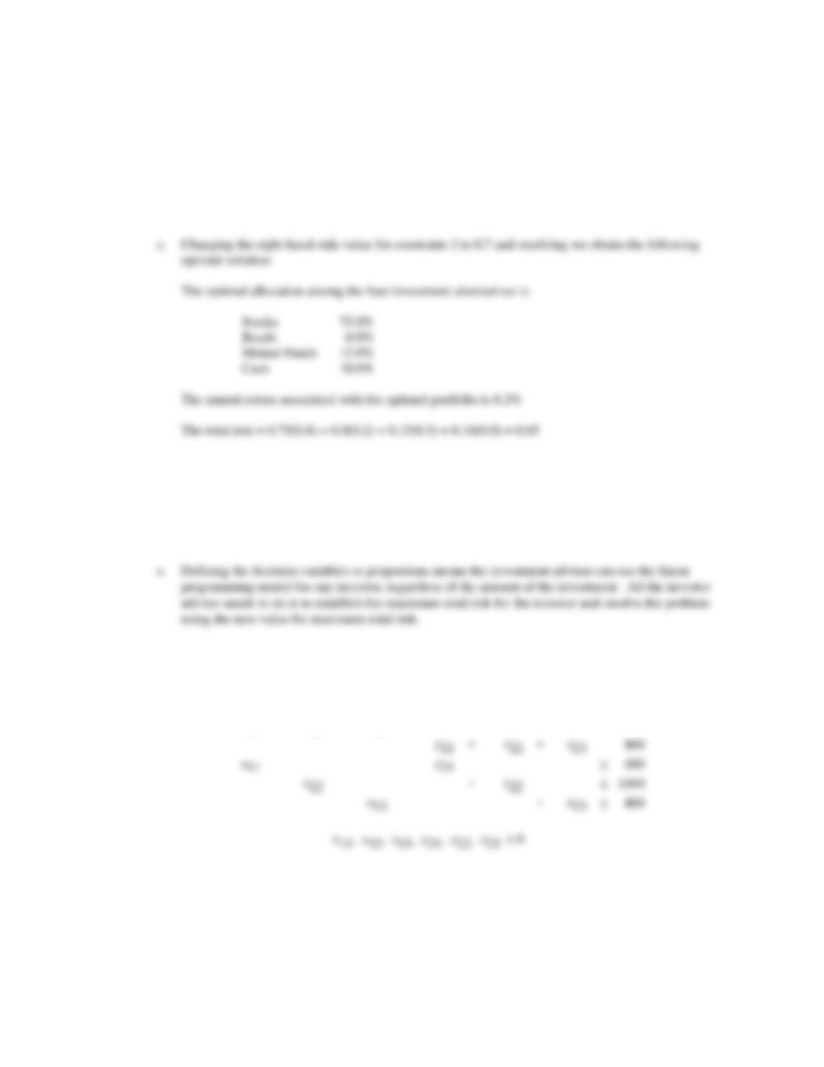
9. Let Xi = the number of call center employees who start work on day i
(i=1 = Monday, i=2=Tuesday…)
Min X1 + X2 + X3 + X4 + X5 + X6 + X7
s.t.
X1 + X4 + X5 + X6 + X7 ≥ 75
X1 + X2 + X5 + X6 + X7 ≥ 50
X1 + X2 + X3 + X6 + X7 ≥ 45
Total Number of Employees = 95
Excess employees: Thursday = 25, Sunday = 10, all others = 0.
Note: There are alternative optima to this problem (Number of employees may differ from
above, but will have objective function value = 95).
10. a. Let S = the proportion of funds invested in stocks
The linear program and optimal solution obtained are as follows:
MAX 0.1S+0.03B+0.04M+0.01C
S.T.
1) 1S + 1B + 1M + 1C = 1
2) 0.8S + 0.2B + 0.3M < 0.4
The optimal allocation among the four investment alternatives is
Stocks 40.9%
The annual return associated with the optimal portfolio is 5.4%
The total risk = 0.409(0.8) + 0.145(0.2) + 0.145(0.3) + 0.300(0.0) = 0.4
Chapter 9
9 – 8
Stocks 0.0%
Bonds 36.0%
Mutual Funds 36.0%
Cash 28.0%
The annual return associated with the optimal portfolio is 2.52%
The total risk = 0.0(0.8) + 0.36(0.2) + 0.36(0.3) + 0.28(0.0) = 0.18
d. Note that a maximum risk of 0.7 was specified for this aggressive investor, but that the risk index for
the portfolio is only 0.65. Thus, this investor is willing to take more risk than the solution shown
above provides. There are only two ways the investor can become even more aggressive: increase
the proportion invested in stocks to more than 75% or reduce the cash requirement of at least 10% so
that additional cash could be put into stocks. For the data given here, the investor should ask the
investment advisor to relax either or both of these constraints.
11. Let xij = units of component i purchased from supplier j
Min
12x11
+
13x12
+
14x13
+
10x21
+
11x22
+
10x23
s.t.
x11
+
x12
+
x13
=
1000
+
+
=
x11
+
x12
+
1000
x13
+
Linear Programming Applications in Marketing, Finance, and Operations Management
9 – 9
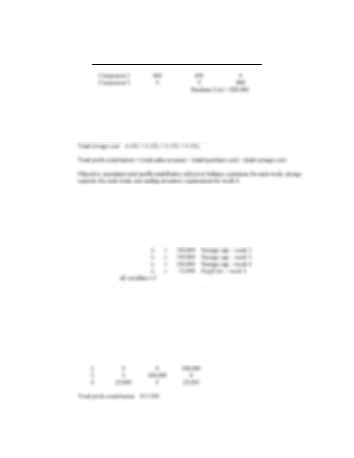
Solution:
Supplier
1
2
3
12. Let Bi = pounds of shrimp bought in week i, i = 1,2,3,4
Si = pounds of shrimp sold in week i, i = 1,2,3,4
Ii = pounds of shrimp held in storage (inventory) in week i
Total purchase cost = 6.00B1 + 6.20B2 + 6.65B3 + 5.55B4
Max 6.00S1 + 6.20S2 + 6.65S3 + 5.55S4 – 6.00B1 – 6.20B2 – 6.65B3 – 5.55B4 – 0.15I1 – 0.15I2 –
0.15I3 – 0.15I4
s.t.
20,000
+
B1
–
S1
=
I1
Balance eq. – week 1
I1
+
B2
–
S2
=
I2
Balance eq. – week 2
I2
+
B3
–
S3
=
I3
Balance eq. – week 3
I3
+
B4
–
S4
=
I4
Balance eq. – week 4
I1
100,000
Storage cap. – week 1
I2
100,000
Storage cap. – week 2
I3
100,000
Storage cap. – week 3
I4
100,000
Storage cap. – week 4
I4
Req’d inv. – week 4
Note that the first four constraints can be written as follows:
I1 – B1 + S1 = 20,000
I1 – I2 + B2 – S2 = 0
I2 – I3 + B3 – S3 = 0
I3 – I4 + B4 – S4 = 0
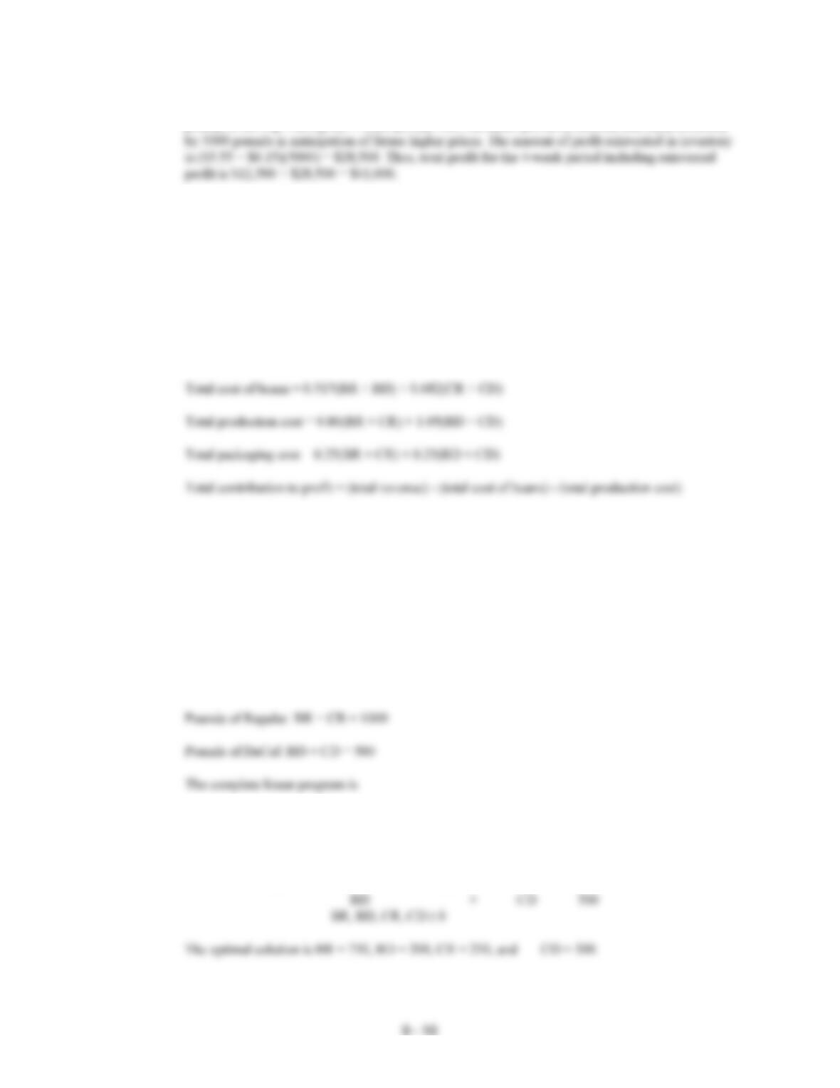
The optimal solution follows:
Week (i)
Bi
Si
Ii
Chapter 9
Note however, ASC started week 1 with 20,000 pounds of shrimp and ended week 4 with 25,000
13. Let BR = pounds of Brazilian beans purchased to produce Regular
BD = pounds of Brazilian beans purchased to produce DeCaf
CR = pounds of Colombian beans purchased to produce Regular
CD = pounds of Colombian beans purchased to produce DeCaf
Type of Bean
Cost per pound ($)
Brazilian
1.10(0.47) = 0.517
Colombian
1.10(0.62) = 0.682
Total revenue = 3.60(BR + CR) + 4.40(BD + CD)
Total contribution to profit = 2.033BR + 2.583BD + 1.868CR + 2.418CD
Regular % constraint
BR = 0.75(BR + CR)
0.25BR – 0.75CR = 0
DeCaf % constraint
BD = 0.40(BD + CD)
0.60BD – 0.40CD = 0
Max
2.033BR
+
2.583BD
+
1.868CR
+
2.418CD
s.t.
0.25BR
–
0.75CR
=
0
0.60BD
–
0.40CD
=
0
BR
+
CR
=
1000
+
=
500
9 – 11
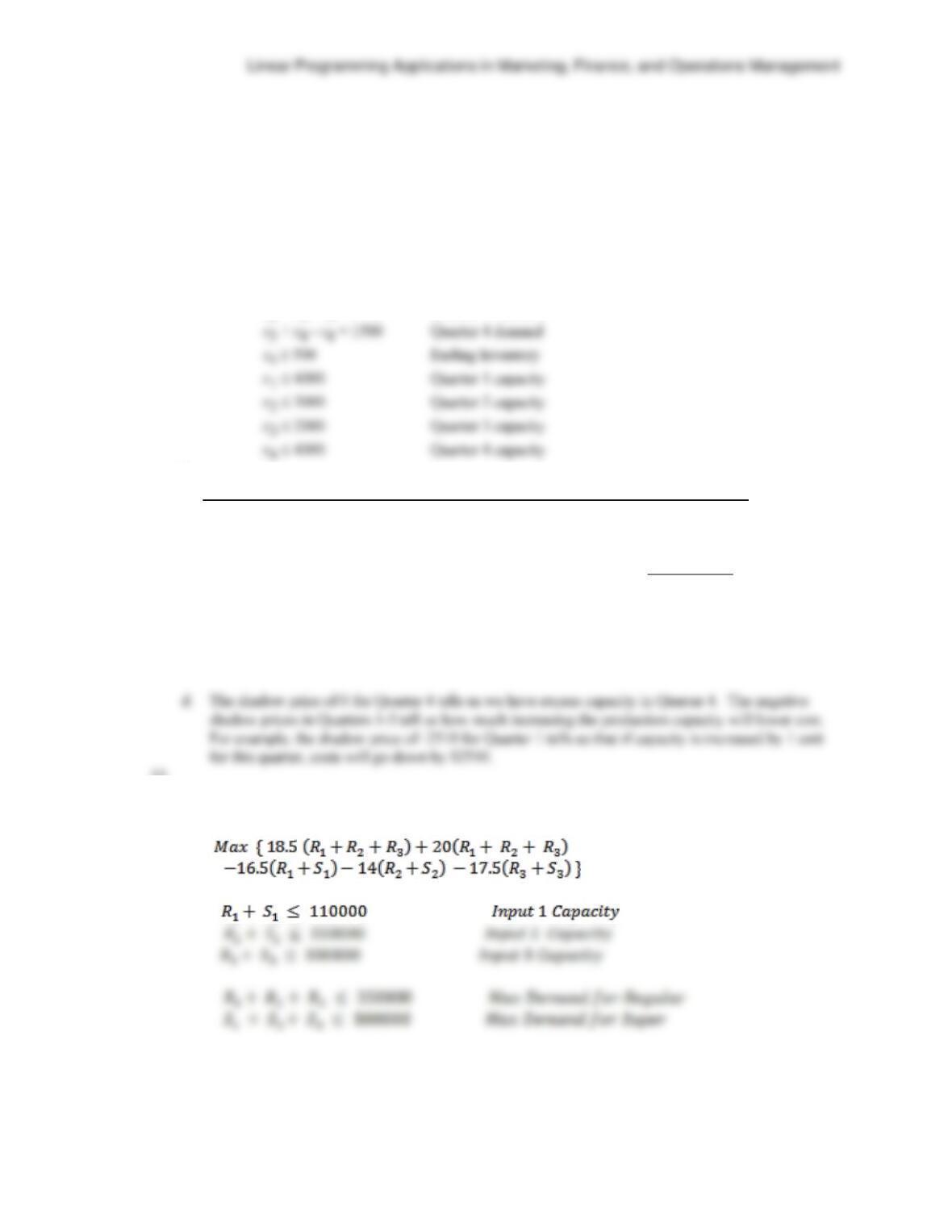
The value of the optimal solution is $3233.75
14. a. Let xi = number of Classic 2l boats produced in Quarter i; i = 1,2,3,4
si = ending inventory of Classic 2l boats in Quarter i; i = 1,2,3,4
Min 10,000x1 + 11,000x2 + 12,100x3 + 13,310x4 + 250s1 + 250s2 + 300s3 + 300s4
s.t.
x1 – s1 = 1900 Quarter 1 demand
s1 + x2 – s2 = 4000 Quarter 2 demand
s2 + x3 – s3 = 3000 Quarter 3 demand
b.
Quarter
Production
Ending Inventory
Cost
1
4000
2100
40,525,000
2
3000
1100
33,275,000
3
2000
100
24,230,000
4
1900
500
25,439,000
$123,469,000
c. The shadow prices tell us how much it would cost if demand were to increase by one additional unit.
For example, in Quarter 2 the shadow price is 12,760; thus, demand for one more boat in Quarter 2
will increase costs by $12,760.
15.
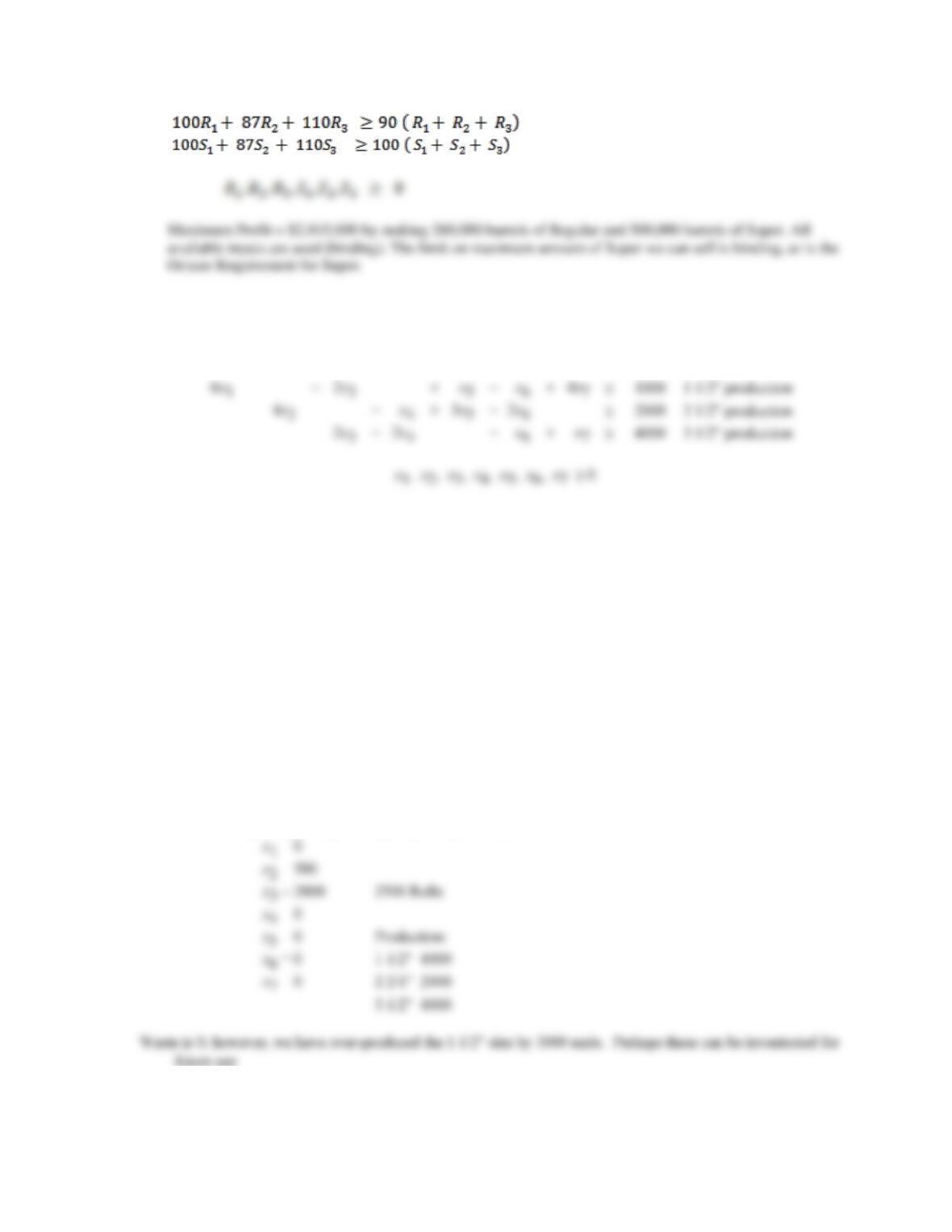
Let Ri = the number of barrels of input i to use to produce Regular, i=1,2,3
Si = the number of barrels of input i to use to produce Super, i=1,2,3
s.t.
Chapter 9
9 – 12
Required Octane Level, Regular
Required Octane Level, Super
16. Let xi = number of 10-inch rolls of paper processed by cutting alternative i; i = 1,2…,7
Min
x1
+
x2
+
x3
+
x4
+
x5
+
x6
+
x7
s.t.
x5
x6
+
x4
+
+
+
+
x6
+
x7
x1 = 0
x2 = 125
x3 = 500 2125 Rolls
x4 = 1500
x5 = 0 Production:
x6 = 0 1 1/2″ 1000
x7 = 0 2 1/2″ 2000
3 1/2″ 4000
Waste: Cut alternative #4 (1/2″ per roll)
750 inches.
b. Only the objective function needs to be changed. An objective function minimizing waste
production and the new optimal solution are given.
Min x1 + 0x2 + 0x3 + 0.5x4 + x5 + 0x6 + 0.5x7
Linear Programming Applications in Marketing, Finance, and Operations Management
9 – 13
c. Minimizing waste may cause you to over-produce. In this case, we used 375 more rolls to generate a
3000 surplus of the 1 1/2″ product. Alternative b might be preferred on the basis that the 3000
surplus could be held in inventory for later demand. However, in some trim problems, excess
17. a. Let FM = number of frames manufactured
FP = number of frames purchased
SM = number of supports manufactured
SP = number of supports purchased
TM = number of straps manufactured
TP = number of straps purchased
Min
38FM
+
51FP
+
11.5SM
+
15SP
+
6.5TM
+
7.5TP
s.t.
+
+
0.8TM
21,000
+
25,200
+
+
1.7TM
40,800
+
5,000
+
10,000
+
5,000
Solution:
Manufacture
Purchase
Frames
5000
0
Supports
2692
7308
Straps
0
5000
b. Total Cost = $368,076.91
Shaping:
d. Nothing, there are already more hours available than are being used.
e. Yes. The current purchase price is $51.00 and the reduced cost of 3.577 indicates that for a purchase
price below $47.423 the solution may improve. Resolving with the coefficient of FP = 45 shows
that 2714 frames should be purchased.
The optimal solution is as follows: