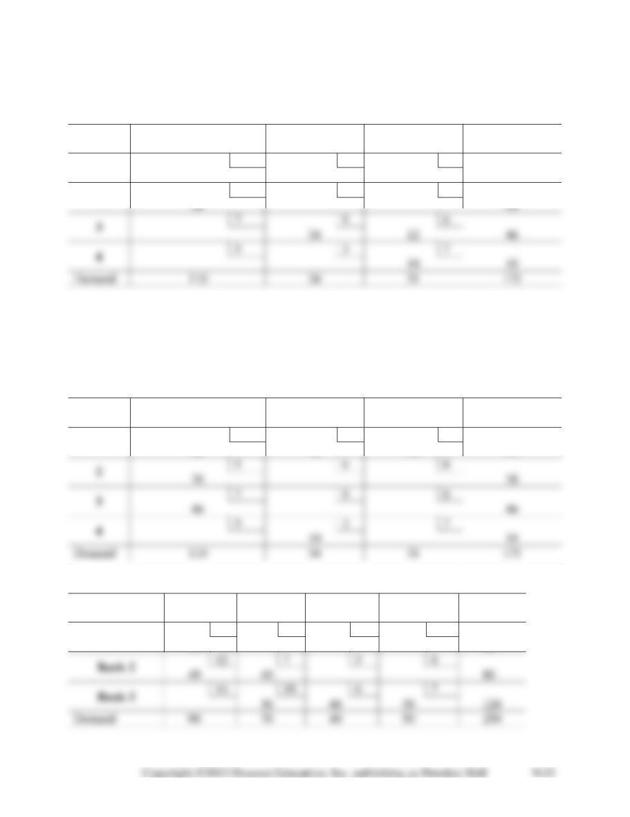
9-25. The initial solution using the northwest corner rule shows that degeneracy exists. The
number of rows plus the number of columns minus 1 is equal to 4 + 3 − 1 = 6, but the number of
occupied squares is only 5.
TO
FROM
A
B
C
Supply
1
8
9
4
72
72
2
5
6
8
38
38
3
7
9
6
34
12
46
4
5
3
7
19
19
Demand
34
31
To solve the problem, a zero will have to be placed in an empty square. The 38 units that were
added to cell 2-A exhausted both the supply and the demand simultaneously, and the normal pat-
tern could not be followed. Therefore, a zero should be placed in either cell 2–B or cell 3-A
which would continue the normal pattern for the northwest corner method. This will enable all
unused paths to be closed. The optimal solution (found after 6 iterations) is shown below with a
total cost = $1,036.
TO
FROM
A
B
C
Supply
1
8
9
4
26
15
31
72
2
5
6
8
38
38
3
7
9
6
46
46
4
5
3
7
19
19
Demand
34
31
9-26. We make the following initial northwest corner assignment:
TO
Hospital
Hospital
Hospital
Hospital
FROM
1
2
3
4
Supply
Bank 1
8
9
11
16
50
50
12
7
5
8
40
40
14
10
6
7
30
40
50
120
Cost = 50($8) + 70($7) + 10($5) + 40($14) + 30($6) + 50($7) = $2,030
Application of the stepping-stone method will yield the following solution in a single itera-
tion. The optimal cost is $2,020.
TO
Hospital
Hospital
Hospital
Hospital
FROM
1
2
3
4
Supply
Bank 1
8
9
11
16
12
7
5
8
14
10
6
7
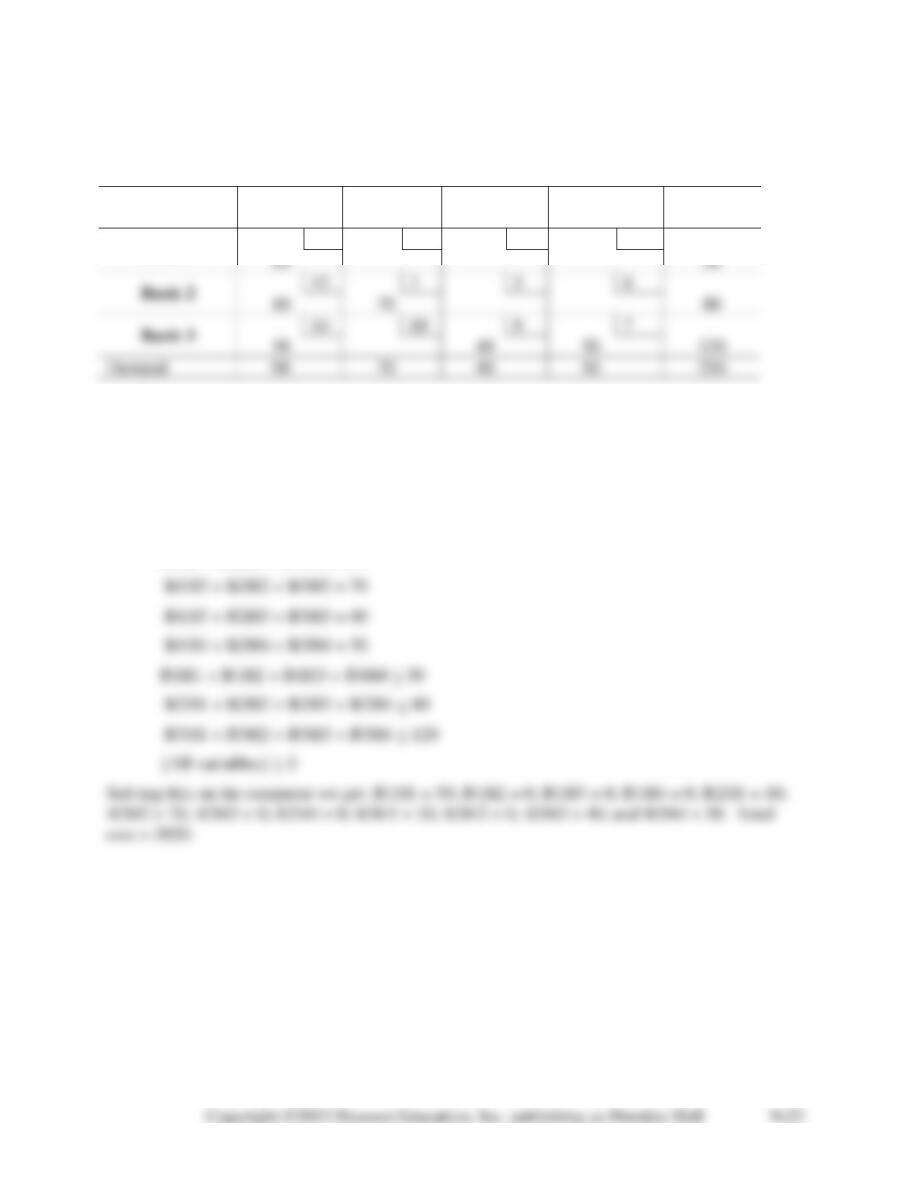
9-27. Let B1H1, B1H2, B1H3, B1H4, B2H1, B2H2, B2H3, B2H4, B3H1, B3H2, B3H3, and
B3H4 represent the containers of blood shipped from blood banks 1, 2, and 3 to hospitals 1, 2, 3,
and 4 respectively. :
Minimize costs: 8B1H1 + 9B1H2 +11B1H3 + 16B1H4 +12B2H1 + 7B2H2 + 5B2H3 +
8B2H4 + 14B3H1 + 10B3H2 + 6B3H3 + 7B3H4
subject to:
B1H1 + B2H1 + B3H1 = 90
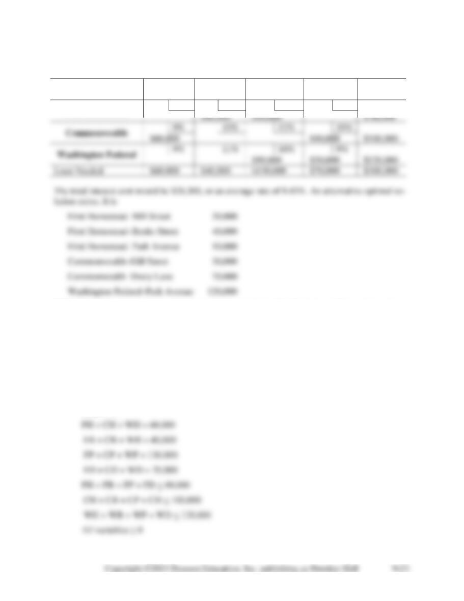
9-28. The optimal solution to the Hall Real Estate decision is shown in the table below.
TO
Drury
Max.
FROM
Hill St.
Banks St.
Park Ave.
Lane
Avail.
First Homestead
8%
8%
10%
11%
9%
10%
12%
10%
9%
11%
10%
9%
Loan Needed
9.29. This problem investigates a borrowing scenario for B. Hall Real Estate Corporation and
models it as a transportation problem. The goal is to borrow all the necessary capital to buy the
four properties while minimizing the total borrowing costs. Let FH, FB, FP, FD, CH, CB, CP,
CD, WH, WB, WP, and WD represent the dollar amounts lent to B. Hall Real Estate from First
Homestead Bank, Commonwealth Bank, and Washington Federal Bank towards the purchase of
the properties located at Hill Street, Banks Street, Park Avenue, and Drury Lane respectively.
The associated linear program can then be formulated as follows:
Minimize costs: 8FH + 8FB + 10FP + 11FD +9CH + 10CB + 12CP + 10CD + 9WH +
11WB + 10WP + 9WD
subject to:
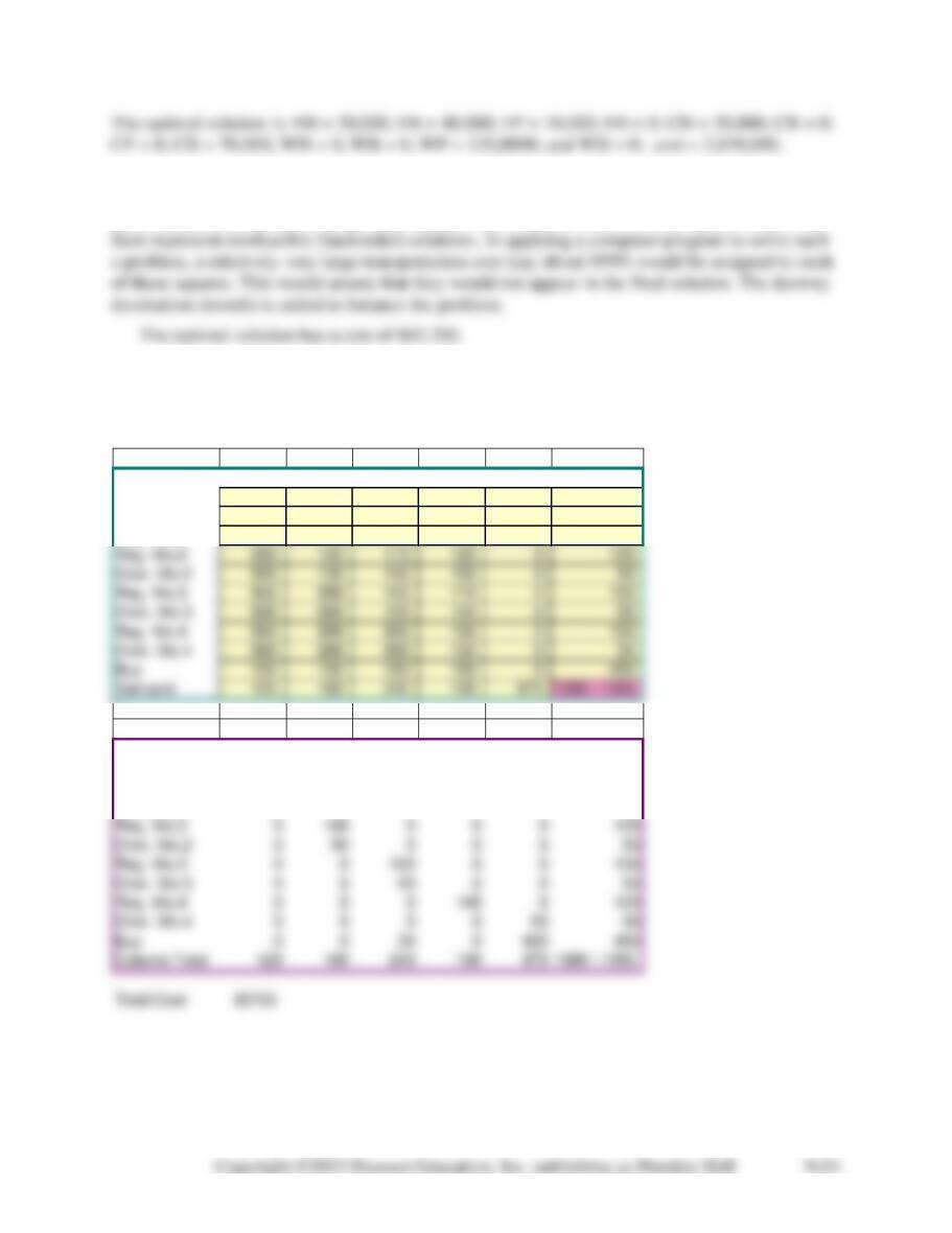
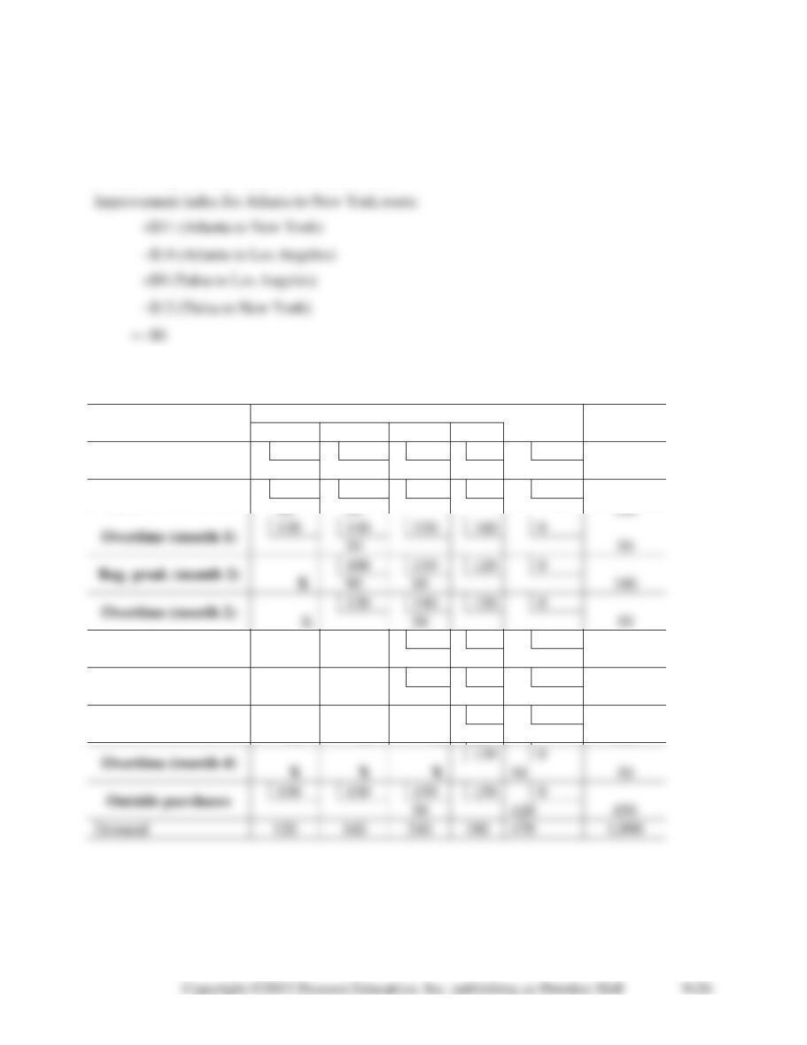
9-30. Mehta’s production smoothing problem is a good exercise in the formulation of transpor-
tation problems and applying them to real-world issues. The problem may be set up as a trans-
portation problem as shown in the table entitled Table for Problem 9-30. All squares with Xs in
The costs for the beginning inventory in months 1, 2, 3, and 4 could be 0, 10, 20, and 30 re-
spectively if the carrying cost for the beginning inventory has already been considered. The solu-
tion is the same but the cost would be $65,300.
Data
COSTS Month 1 Month 2 Month 3 Month 4 Dummy Supply
Beginning 10 20 30 40 040
Reg. Mo.1 100 110 120 130 0100
Over. Mo.1 130 140 150 160 050
Shipments
Shipments Month 1 Month 2 Month 3 Month 4 Dummy Row Total
Beginning 40 0 0 0 0 40
Reg. Mo.1 40 060 0 0 100
Over. Mo.1 40 10 0 0 0 50
9-31. There are several ways to formulate this as a linear program. Let RM1, RM2, RM3, and
RM4, OM1, OM2, OM3, and OM4 represent the amount produced on regular time and on over-
time in months 1-4 respectively. Let E0 = the amount in inventory at the beginning of month 1.
Let E1, E2, E3, and E4 be the amount left in inventory at the end of month 1, 2, 3, and 4 respec-
tively. Let B1, B2, B3, and B4 represent the amount bought in month 1, 2, 3, and 4 respectively.
The associated linear program can then be formulated as follows:
Minimize cost: 100RM1 + 100RM2 + 100RM3 + 100RM4 + 130OM1 + 130OM2 +
130OM3 + 130OM4 + 10E0 +10E1 + 10E2 + 10E3 + 10E4 + 150B1 + 150B2+ 150B3+
150B4
subject to:
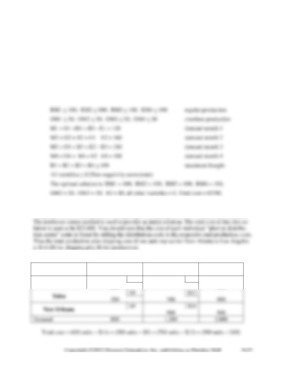
9-32. To determine which new plant will yield the lowest cost for Ashley in combination with
the existing plants, we need to solve two transportation problems. We begin by setting up a
transportation table that represents the opening of the third plant in New Orleans (see the table).
Table for Problem 9-32
TO
Production
FROM
Los Angeles
New York
Capacity
Atlanta
$14
$11
600
600
$9
$12
200
700
900
$9
$10
500
500
Demand
800
= $8,400 + $1,800 + $8,400 + $5,000
= $23,600
Is this initial solution optimal? We once again employ the stepping-stone method to test it and to
compute improvement indices for unused routes.
Table for Problem 9-30
Destination (Month)
Sources
1
2
3
4
Dummy
Capacity
Beginning inv.
10
20
30
40
0
40
40
Reg. prod. (month 1)
100
110
120
130
0
80
100
130
140
150
160
0
Reg. prod. (month 2)
100
110
120
0
X
10
100
130
140
150
0
X
50
50
Reg. prod. (month 3)
100
110
0
X
X
100
100
Overtime (month 3)
130
140
0
X
X
50
50
Reg. prod. (month 4)
100
0
X
X
X
100
100
130
0
X
X
X
50
50
150
150
150
150
0
30
420
450
Demand
120
160
240
100
470
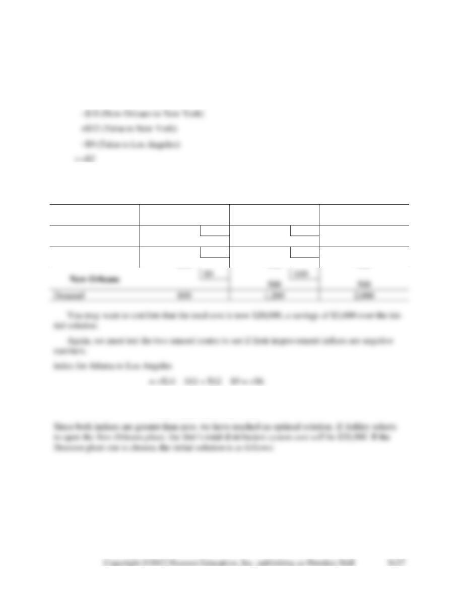
9-32. (continued)
Improvement index for New Orleans to Los Angeles route:
+$9 (New Orleans to Los Angeles)
Since the firm can save $6 for every unit it ships from Atlanta to New York, it will want to im-
prove the initial solution and send as many as possible (600 in this case) on this currently unused
route.
TO
Production
FROM
Los Angeles
New York
Capacity
Atlanta
$14
$11
600
600
Tulsa
$9
$12
800
100
900
$9
$10
500
500
Demand
800
index for New Orleans to Los Angeles
= +$9 − $10 + $12 − $9 = +$2
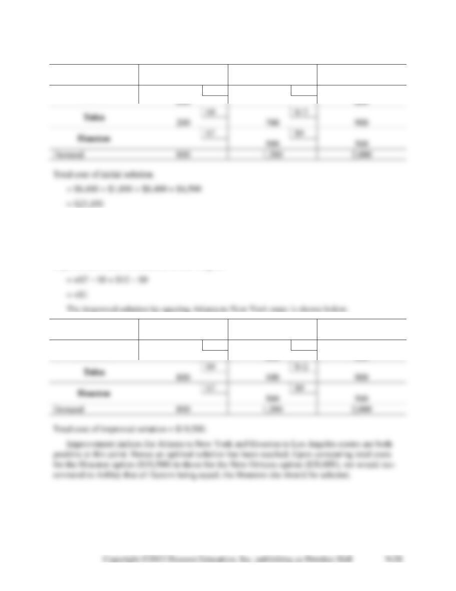
TO
FROM
Los Angeles
New York
Capacity
Atlanta
$14
$11
600
600
$9
$12
200
700
900
$7
$9
500
500
Demand
800
Improvement index for Atlanta to New York
= +$11 − $14 + $9 − $12
= −$6
Improvement index for Houston to Los Angeles
The improved solution by opening Atlanta to New York route is shown below.
TO
Production
FROM
Los Angeles
New York
Capacity
Atlanta
$14
$11
600
600
$9
$12
800
100
900
$7
$9
500
500
Demand
800
9-33. For this analysis, we must consider two formulations. For both of them let A1, A2, T1, T2,
N1, N2, H1, and H2 represent the carriers delivered from Atlanta, Tulsa, New Orleans, and Hou-
ston to Los Angeles (1) and New York (2) respectively. The first linear program for the New Or-
leans option can then be formulated as follows:
Minimize costs: 14A1 + 11A2 + 9T1 +12T2 + 9N1 + 10N2
subject to:
A1 + A2 < 600
The optimal solution is: A1 = 0; A2 = 600; T1 = 800; T2 = 100; N1 = 0; N2 = 500; cost =
20,000.The second alternative for Houston can be formulated as follows:
Minimize costs: 14A1 + 11A2 + 9T2 +12T2 + 7H1 + 9H2
subject to:
A1 + A2 < 600
9-34. Considering Fontainebleau, we have:
South
Pacific
Canada
America
Rim
Europe
Capacity
Waterloo
60
70
75
75
4,000
4,000
8,000
55
55
40
70
2,000
2,000
60
50
65
70
5,000
5,000
75
80
90
60
4,000
5,000
9,000
Market Demand
4,000
5,000
10,000
Optimal cost = $1,530,000.
Considering Dublin, we have the following initial northwest corner solution:
South
Pacific
Canada
America
Rim
Europe
Capacity
Waterloo
60
70
75
75
4,000
4,000
8,000
55
55
40
70
1,000
1,000
2,000
60
50
65
70
5,000
5,000
70
75
85
65
4,000
5,000
9,000
Market Demand
4,000
5,000
10,000
5,000
Final solution:
South
Pacific
Canada
America
Rim
Europe
Capacity
Waterloo
60
70
75
75
4,000
4,000
8,000
Pusan
55
55
40
70
2,000
2,000
60
50
65
70
5,000
5,000
70
75
85
65
4,000
5,000
9,000
Market Demand
4,000
5,000
10,000
5,000
Optimal cost = $1,535,000.
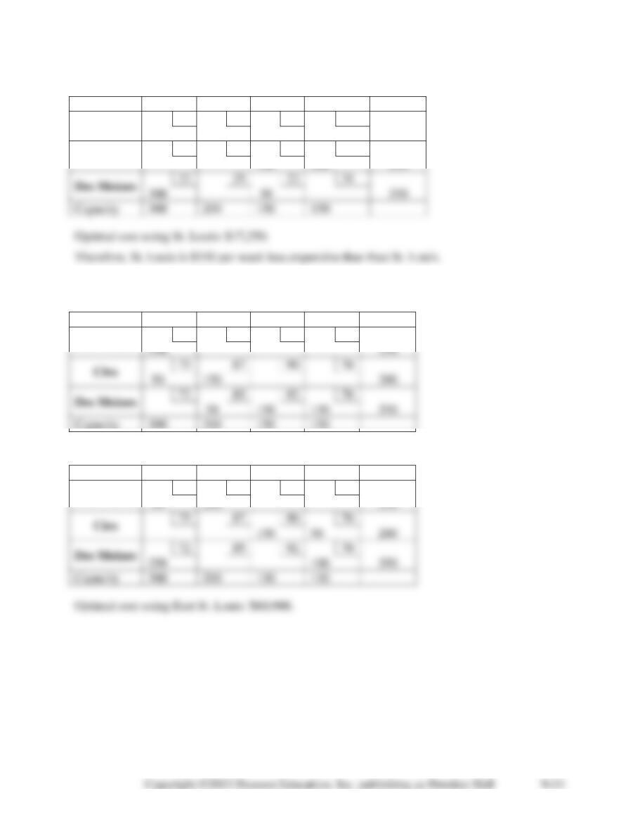
There is no difference in the routing of shipments, but the Fontainebleau location is $5,000 less expensive than the Dublin location. As
9-35. Considering East St. Louis, we have:
Initial solution—northwest corner rule:
Decatur
Minn.
C’dale
E. St. L.
Demand
Blue Earth
20
17
21
29
250
250
25
27
20
30
150
200
22
25
22
30
150
150
350
Capacity
300
200
150
150
800
Optimal solution:
Decatur
Minn.
C’dale
E. St. L.
Demand
Blue Earth
20
17
21
29
50
200
250
Ciro
25
27
20
30
150
50
200
Des Moines
22
25
22
30
250
100
350
Capacity
300
200
150
150
800
Optimal cost using East St. Louis: $17,400.
20
17
21
27
25
27
20
28
22
25
22
31
Capacity
Optimal solution:
Decatur
Minn.
C’dale
St. Louis
Demand
Blue Earth
20
17
21
27
200
50
250
Ciro
25
27
20
28
100
100
200
22
25
22
31
300
50
350
Capacity
300
200
150
150
9-36. Considering East St. Louis, we have:
Initial solution—northwest corner rule:
Decatur
Minn.
C’dale
E. St. L.
Demand
Blue Earth
70
77
91
69
250
250
75
87
90
70
50
150
200
72
85
92
70
50
150
150
350
Capacity
300
200
150
150
Optimal solution:
Decatur
Minn.
C’dale
E. St. L.
Demand
Blue Earth
70
77
91
69
50
200
250
Ciro
75
87
90
70
150
50
200
72
85
92
70
250
100
350
Capacity
300
200
150
150
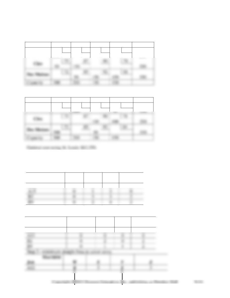
Considering St. Louis, we have:
Initial solution—northwest corner rule:
Decatur
Minn.
C’dale
St. Louis
Demand
Blue Earth
70
77
91
77
250
250
75
87
90
78
150
200
72
85
92
81
150
350
Capacity
300
200
150
Optimal solution:
Decatur
Minn.
C’dale
St. Louis
Demand
Blue Earth
70
77
91
77
200
75
87
90
78
100
100
72
85
92
81
300
Capacity
300
200
150
150
Therefore, when considering production costs, East St. Louis is $1,350 per week less expensive
than St. Louis.
9-37. Step 1—row subtraction:
MACHINE
JOB
W
X
Y
Z
A12
0
4
6
3
A15
0
1
3
0
0
3
3
2
0
2
4
2
Column subtraction:
MACHINE
JOB
W
X
Y
Z
A12
0
3
3
3
A15
0
0
0
0
0
2
0
2
0
1
1
2
MACHINE
A15
0
0
0
0
B2
0
2
0
2
B9
0
1
1
2
Step 3—subtract the smallest uncovered number from all the uncovered numbers and add it to
numbers at both intersections of two lines:
MACHINE
JOB
W
X
Y
Z
A12
0
2
3
2
A15
1
0
1
0
B2
0
1
0
1
B9
0
0
1
1
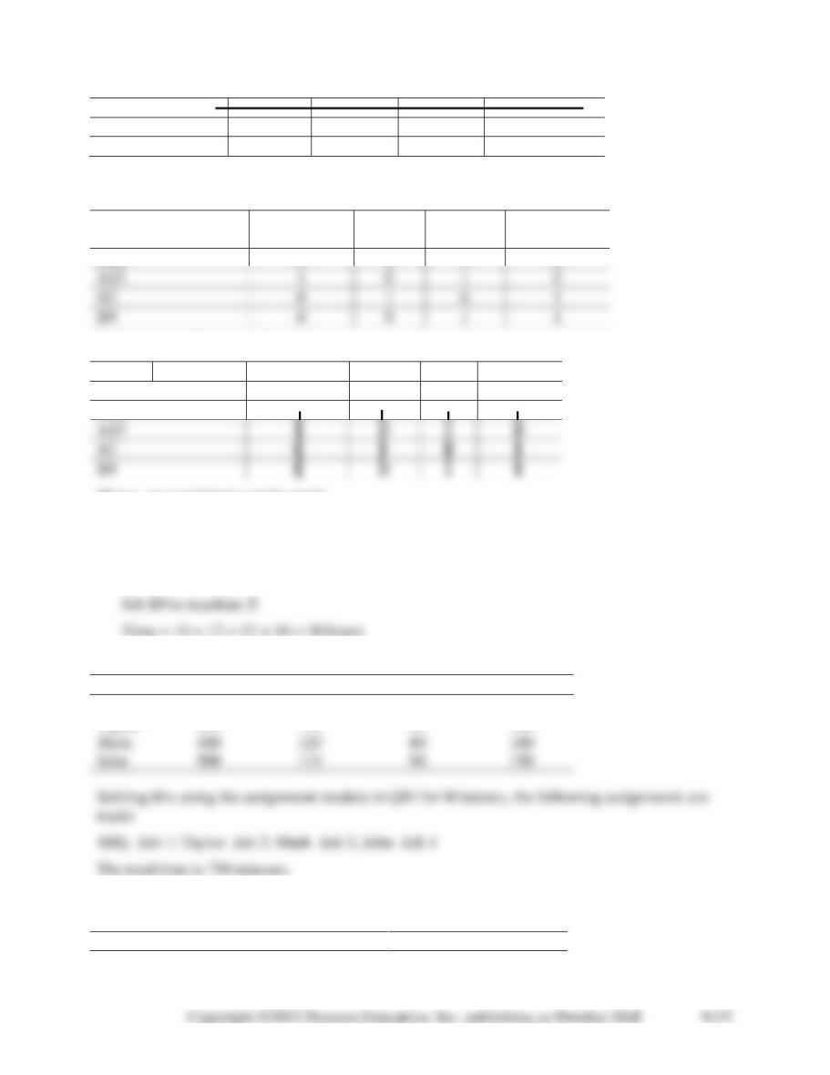
Return to step 2—cover all zeros:
MACHINE
JOB
W
X
Y
Z
A12
0
2
3
2
A15
1
0
1
0
B2
0
1
0
1
B9
0
0
1
1
Hence, an assignment can be made:
Job A12 to machine W
Job A15 to machine Z
Job B2 to machine Y
9-38. The initial table used for the assignment problem is:
Job 1
Job 2
Job 3
Job 4
Billy
400
90
60
120
Taylor
650
120
90
180
Mark
480
120
80
180
John
500
110
90
150
9-39. For the prohibited route where no assignment may be made, a very high cost (10,000
miles) used to prevent anything from being assigned here. The initial assignment table is:
Kansas City
Chicago
Detroit
Toronto
Seattle
1500
1730
1940
2070