Chapter 9: Forecasting
Introduction to Operations & Supply Chain Management (Bozarth & Handfield, 3rd Ed.)
DIRECTIONS Enter the instructor-provided 4-digit number to generate the homework key.
Name: *** KEY ***
Problem 1 Develop a single exponential smoothing forecast for Periods 1 through 9, using the data below.
Each time you develop a forecast, round your answer off to a whole number (ex. – 2012.6 = 2013).
Use a smoothing constant value of 0.3.
Actual
Week Demand Forecast
14545 4500
24091 4514
Chapter 9: Forecasting 2
*** KEY ***
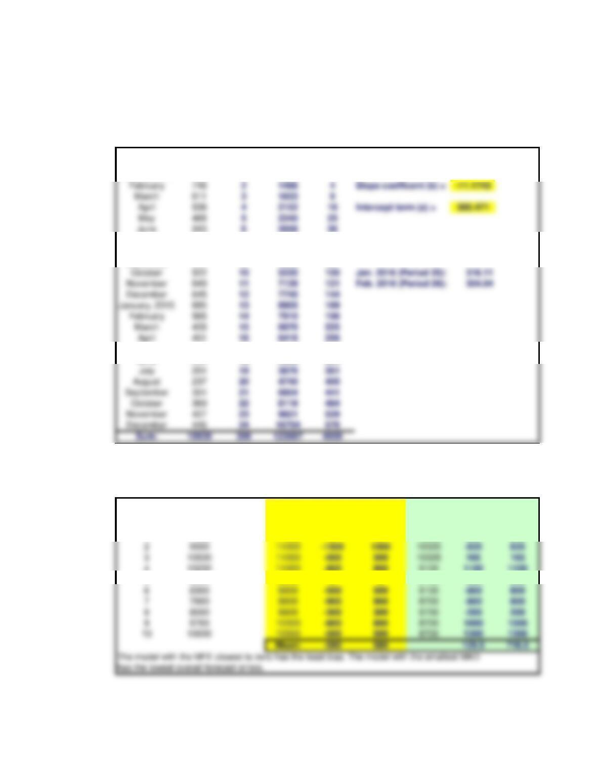
Problem 2 Use regression analysis to develop a time series forecasting model for the data below,
and develop seasonal indices for each month.
Use your regression model to forecast develop forecasts for January and February of 2016.
Y
Month Demand X X*Y X^2 y = a + b(Period)
January, 2014 636 1636 1
July 283 71981 49
August 328 82624 64 Forecasts:
September 454 94086 81
January, 2015 685 13 8905 169
May 346 17 5882 289
June 252 18 4536 324
August 237 20 4740 400
September 324 21 6804 441
Problem 3 Calculate the mean forecast error and mean absolute deviation for the two forecast models
shown below. Which model has the least bias? Which model has the lowest overall forecast errors?
Actual Forecast Forecast
Period Demand Model 1 Model 2
FE AD FE AD
111000 11000 0 0 10335 665 665
29500 11000 -1500 1500 10335 -835 835
310500 11000 -500 500 10335 165 165
410200 11000 -800 800 9100 1100 1100
58800 8800 0 0 9100 -300 300
68300 8800 -500 500 9100 -800 800
77900 8800 -900 900 8700 -800 800
88500 8800 -300 300 8700 -200 200
99700 10500 -800 800 8700 1000 1000
May 468 52340 25
June 343 62058 36