Chapter 9
OPTIMAL SOLUTION
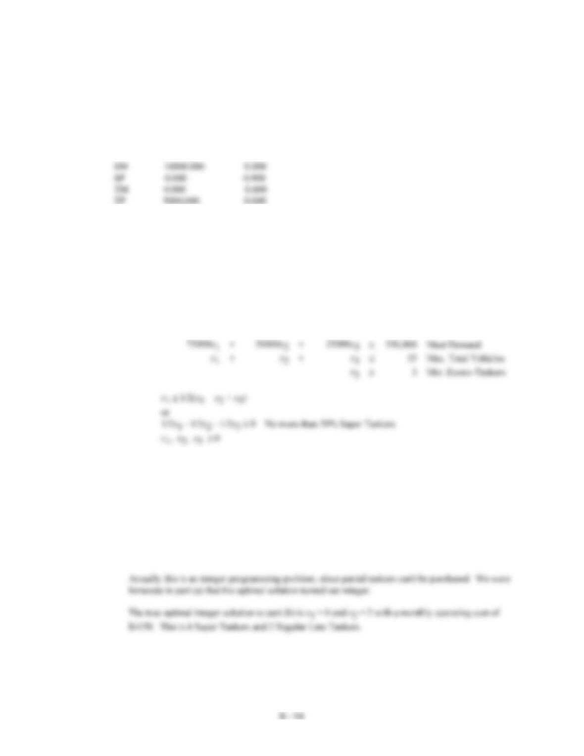
Objective Function Value = 361500.000
Variable Value Reduced Costs
————– ————— ——————
FM 2285.714 0.000
FP 2714.286 0.000
18. a. Let x1 = number of Super Tankers purchased
x2 = number of Regular Line Tankers purchased
x3 = number of Econo-Tankers purchased
Min
550x1
+
425x2
+
350x3
s.t.
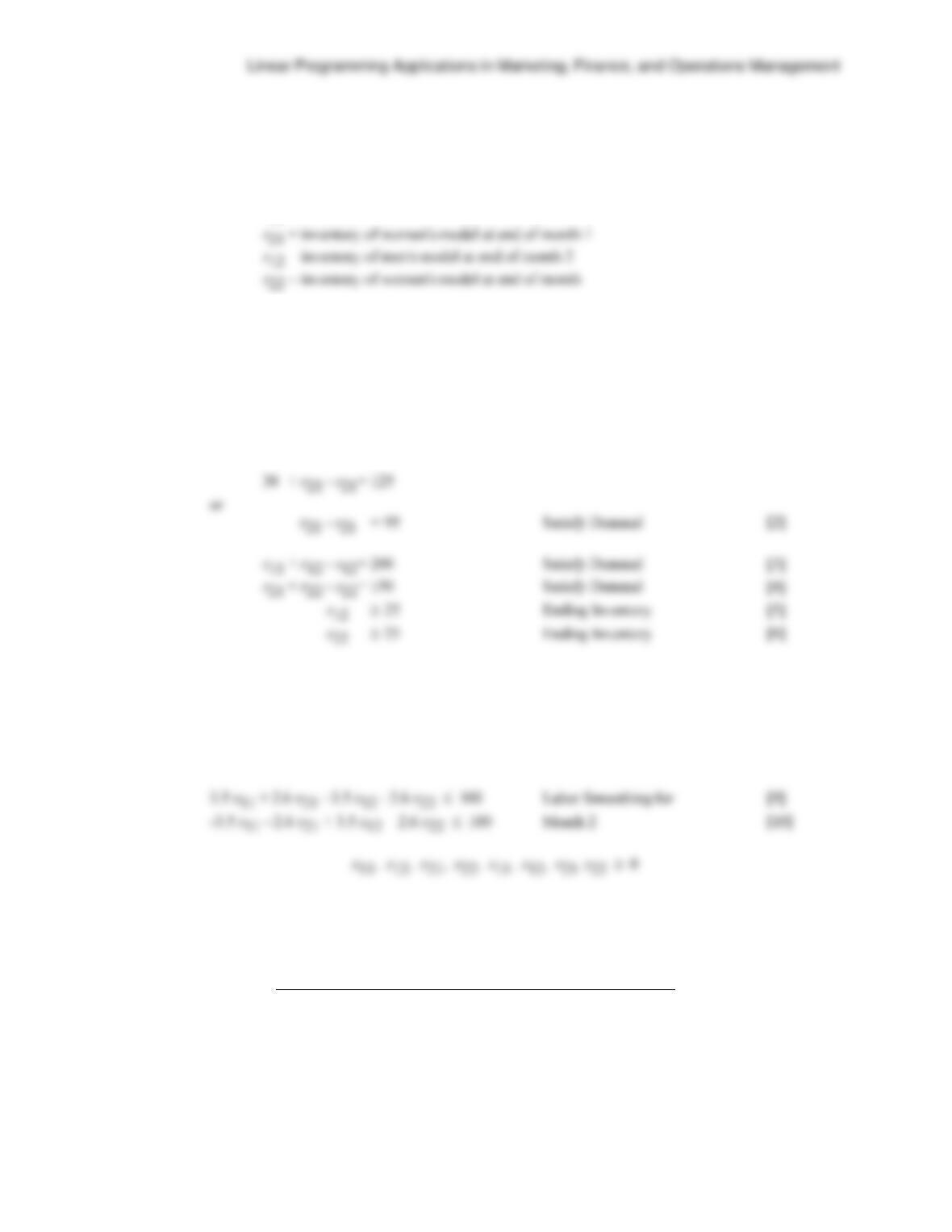
6700x1
+
55000x2
+
4600x3
600,000
Budget
15(5000)x1
+
20(2500)x2
+
25(1000)x3
550,000
or
+
50000x2
+
550,000
+
+
Solution: 5 Super Tankers, 2 Regular Tankers, 3 Econo-Tankers
Total Cost: $583,000
Monthly Operating Cost: $4,650
b. The last two constraints in the formulation above must be deleted and the problem resolved.
The optimal solution calls for 7 1/3 Super Tankers at an annual operating cost of $4033. However,
since a partial Super Tanker can’t be purchased we must round up to find a feasible solution of 8
Super Tankers with a monthly operating cost of $4,400.
9 – 15
19. a. Let x11 = amount of men’s model in month 1
x21 = amount of women’s model in month 1
x12 = amount of men’s model in month 2
x22 = amount of women’s model in month 2
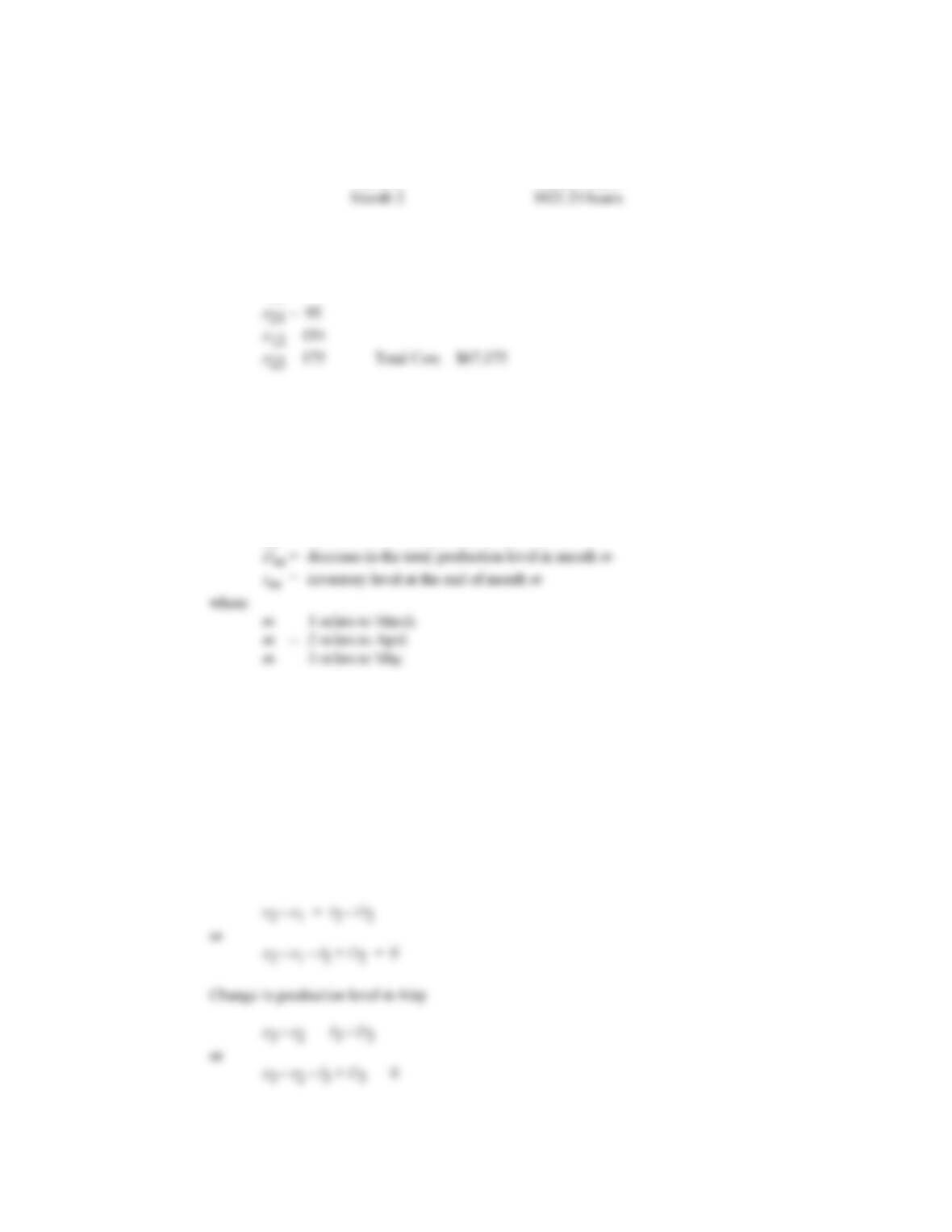
s11 = inventory of men’s model at end of month 1
The model formulation for part (a) is given.
Min 120x11 + 90x21 + 120x12 + 90x22 + 2.4s11 + 1.8s21 + 2.4s12 + 1.8s22
s.t.
20 + x11 – s11 = 150
or
x11 – s11 = 130 Satisfy Demand [1]
Labor Hours: Men’s = 2.0 + 1.5 = 3.5
Women’s = 1.6 + 1.0 = 2.6
3.5 x11 + 2.6 x21 900 Labor Smoothing for [7]
3.5 x11 + 2.6 x21 1100 Month 1 [8]
The optimal solution is to produce 193 of the men’s model in month 1, 162 of the men’s model in
month 2, 95 units of the women’s model in month 1, and 175 of the women’s model in month 2.
Total Cost = $67,156
Inventory Schedule
Month 1
63 Men’s
0 Women’s
Month 2
25 Men’s
25 Women’s
Chapter 9
9 – 16
Labor Levels
Previous month
1000.00 hours
Month 1
922.25 hours
b. To accommodate this new policy the right-hand sides of constraints [7] to [10] must be changed to
950, 1050, 50, and 50 respectively. The revised optimal solution is given.
x11 = 201
We produce more men’s models in the first month and carry a larger men’s model inventory; the
added cost however is only $19. This seems to be a small expense to have less drastic labor force
fluctuations. The new labor levels are 1000, 950, and 994.5 hours each month. Since the added cost
is only $19, management might want to experiment with the labor force smoothing restrictions to
enforce even less fluctuations. You may want to experiment yourself to see what happens.
20. Let xm = number of units produced in month m
Im = increase in the total production level in month m
Min 1.25 I1 + 1.25 I2 + 1.25 I3 + 1.00 D1 + 1.00 D2 + 1.00 D3
s.t.
Change in production level in March
x1 – 10,000 = I1 – D1
or
x1 – I1 + D1 = 10,000
Change in production level in April
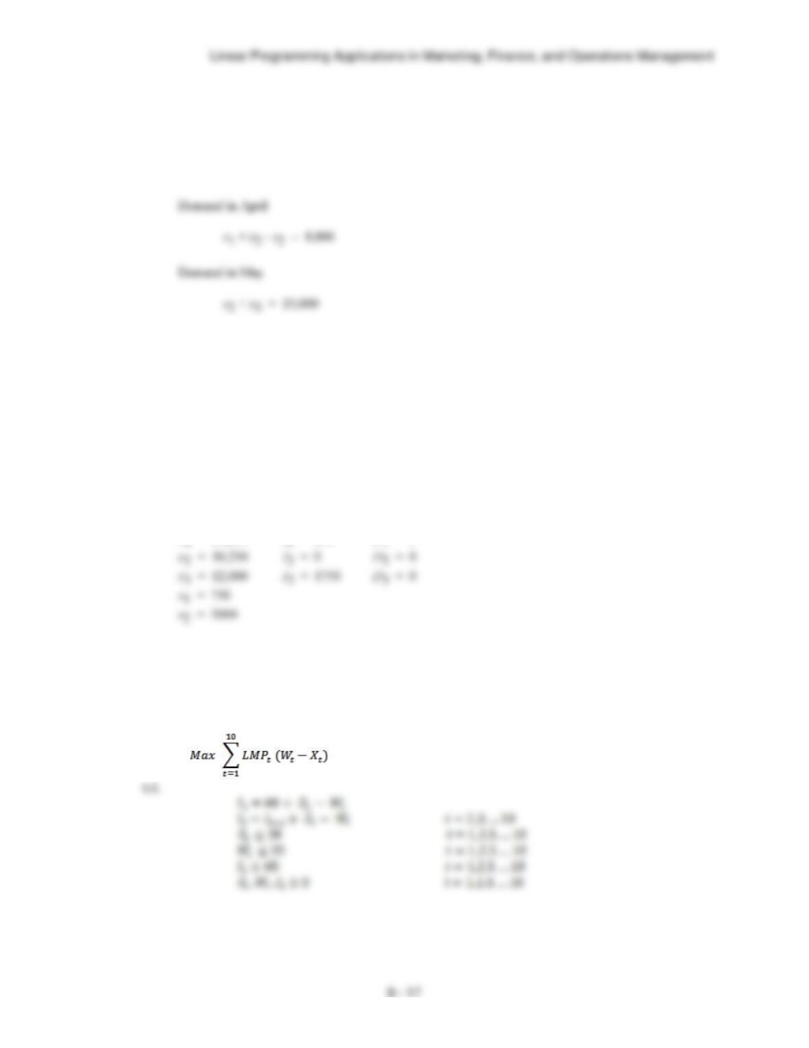
Demand in March
2500 + x1 – s1 = 12,000
or
x1 – s1 = 9,500
Inventory capacity in March
s1 3,000
Inventory capacity in April
s2 3,000
Optimal Solution:
Total cost of monthly production increases and decreases = $2,500
21. a.
Let LMPt = the Locational Marginal Price for period t (data) t = 1,2,3,…10
Xt = the amount to buy (inject into the battery) in period t, t = 1,2,3,…10
Wt = the amount to sell (withdraw from the battery) in period t, t = 1,2,3,…10
It = the battery level at the end of period t, t = 1,2,3,…10
Chapter 9
9 – 18
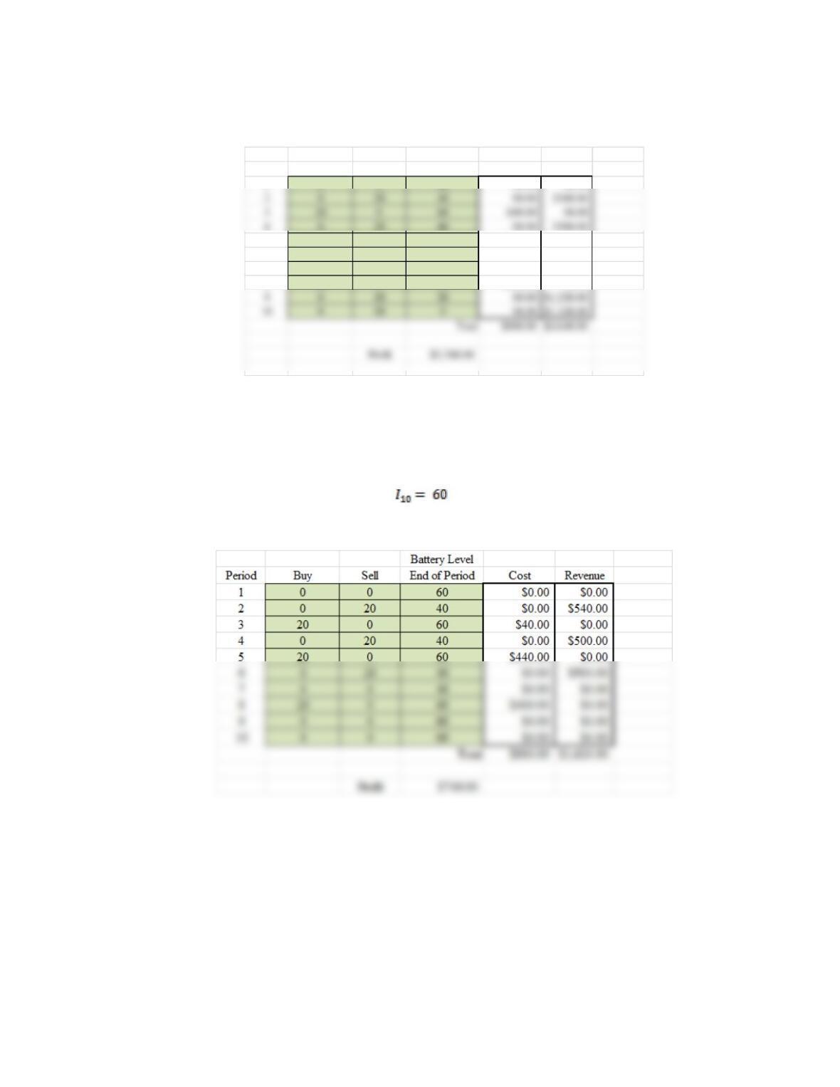
The solution is:
Battery Level
Period Buy Sell End of Period Cost Revenue
520 060 $440.00 $0.00
6 0 20 40 $0.00 $580.00
7 0 20 20 $0.00 $480.00
The maximal achievable profit is $3,760.
b. The ending inventory in period 10 is 0 because it has a positive cost and no benefit (since the model
knows nothing of periods 11 onward).
To ensure an ending inventory in period 10 of 60 kWh, add the constraint:
Optimal profit drops dramatically to $740.
Linear Programming Applications in Marketing, Finance, and Operations Management
9 – 19
c.
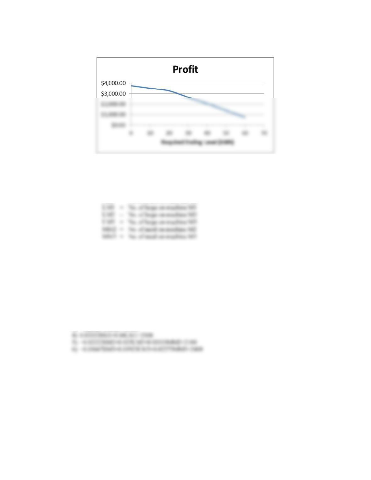
The decrease in profit is much higher after an ending requirement of 20. So, to be conservative, require 20
kWh as the ending requirement for period 10.
22. Let SM1 = No. of small on machine M1
SM2 = No. of small on machine M2
The formulation and solution follows. Note that constraints 1-3 guarantee that next week’s schedule
will be met and constraints 4-6 enforce machine capacities.
LINEAR PROGRAMMING PROBLEM
MIN 20SM1+24SM2+32SM3+15LM1+28LM2+35LM3+18MM2+36MM3
S.T.
1) 1SM1+1SM2+1SM3>80000
2) +1LM1+1LM2+1LM3>80000
Chapter 9
9 – 20
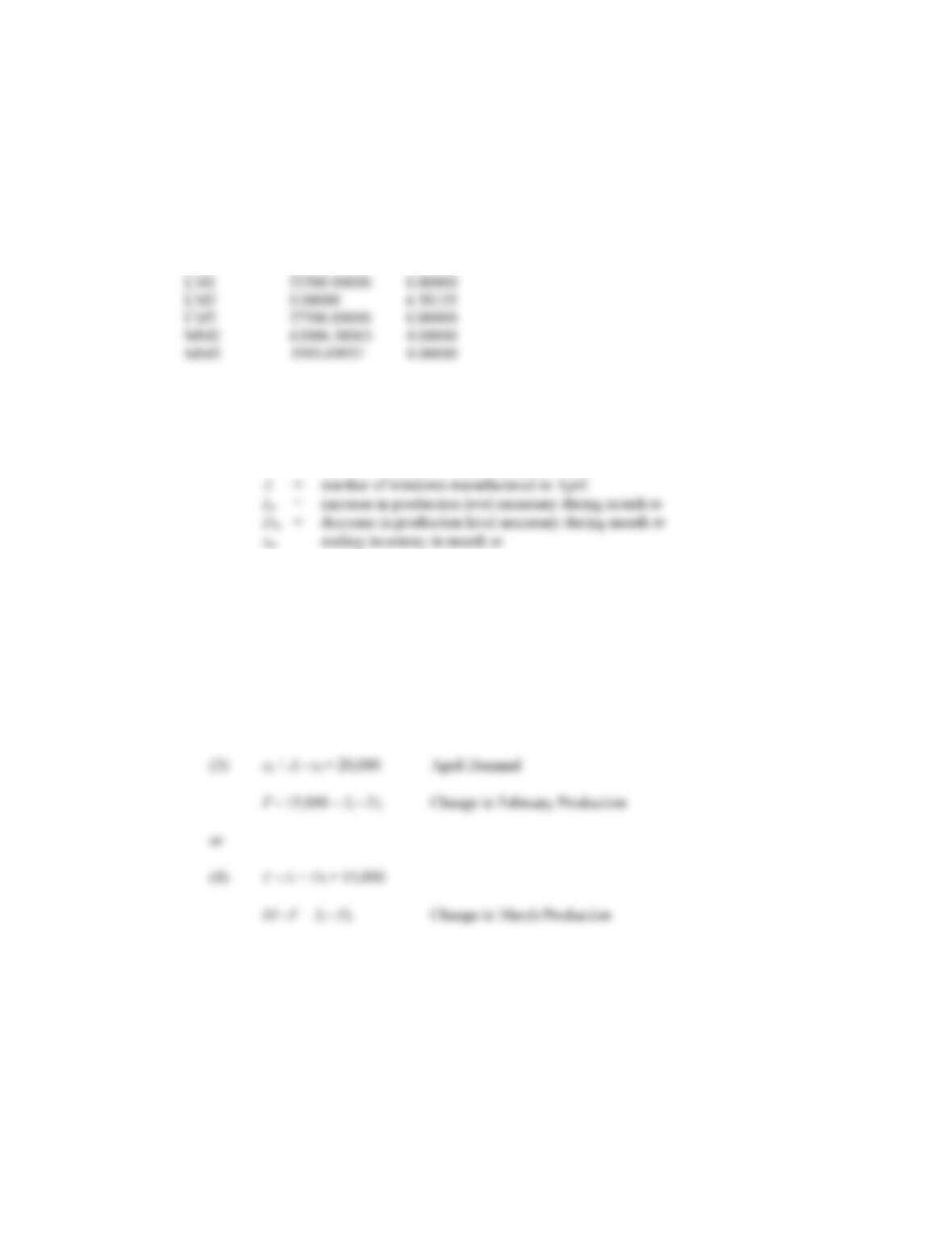
OPTIMAL SOLUTION
Objective Function Value = 5515886.58866
Variable Value Reduced Costs
————– ————— ——————
SM1 0.00000 4.66500
SM2 0.00000 4.00000
SM3 80000.00000 0.00000
Note that 5,515,887 square inches of waste are generated. Machine 3 has 492 minutes of idle
capacity.
23. Let F = number of windows manufactured in February
M = number of windows manufactured in March
Min 1I1 + 1I2 + 1I3 + 0.65D1 + 0.65D2 + 0.65D3
s.t.
9000 + F – s1 = 15,000 February Demand
or
(1) F1 – s1 = 6000
(2) s1 + M – s2 = 16,500 March Demand
or
(5) M – F – I2 + D2 = 0
A – M = I3 – D3 Change in April Production
or
(6) A – M – I3 + D3 = 0
Linear Programming Applications in Marketing, Finance, and Operations Management
9 – 21
(7) F 14,000 February Production Capacity
(8) M 14,000 March Production Capacity
(9) A 18,000 April Production Capacity
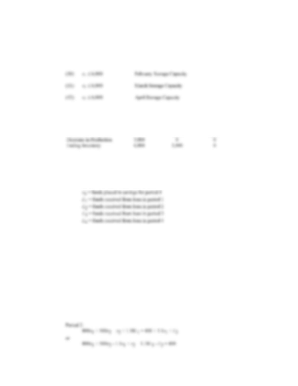
Optimal Solution: Cost = $6,450
February
March
April
Production Level
12,000
14,000
16,500
Increase in Production
0
2,000
2,500
Decrease in Production
3,000
0
0
Ending Inventory
6,000
3,500
0
24. Let x1 = proportion of investment A undertaken
x2 = proportion of investment B undertaken
s1 = funds placed in savings for period 1
s2 = funds placed in savings for period 2
s3 = funds placed in savings for period 3
Objective Function:
In order to maximize the cash value at the end of the four periods, we must consider the value of
investment A, the value of investment B, savings income from period 4, and loan expenses for
period 4.
Max 3200x1 + 2500x2 + 1.1s4 – 1.18L4
Constraints require the use of funds to equal the source of funds for each period.
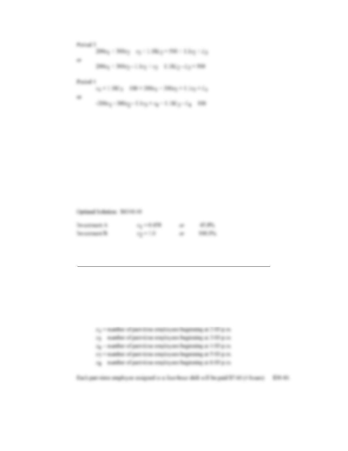
Period 1:
1000x1 + 800x2 + s1 = 1500 + L1
or
1000x1 + 800x2 + s1 – L1 = 1500
Chapter 9
9 – 22
Limits on Loan Funds Available
L1 200
L2 200
L3 200
L4 200
Proportion of Investment Undertaken
x1 1
x2 1
Savings/Loan Schedule:
Period 1
Period 2
Period 3
Period 4
Savings
242.11
—
—
341.04
Loan
—
200.00
127.58
—
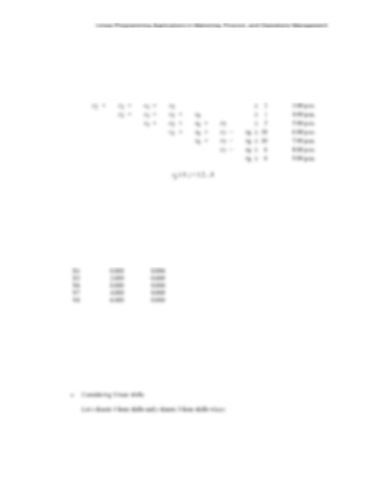
25. Let x1 = number of part-time employees beginning at 11:00 a.m.
x2 = number of part-time employees beginning at 12:00 p.m.
x3 = number of part-time employees beginning at 1:00 p.m.
9 – 23
Min
30.4x1
+
30.4x2
+
30.4x3
+
30.4x4
+
30.4x5
+
30.4x6
+
30.4x7
+
30.4x8
Part-Time
Employees Needed
s.t.
x1
8
11:00 a.m.
x1
+
x2
8
12:00 p.m.
x1
+
x2
+
x3
7
1:00 p.m.
x1
+
x2
+
x3
+
x4
1
2:00 p.m.
x2
x3
x4
+
x5
2
x3
+
x4
+
x5
+
x6
1
4:00 p.m.
x4
+
x5
+
x6
+
x7
5
5:00 p.m.
x5
x6
x7
+
x8
x6
+
x7
+
x8
7:00 p.m.
x7
+
x8
6
x8
6
9:00 p.m.
Full-time employees reduce the number of part-time employees needed.
OPTIMAL SOLUTION
Objective Function Value = 608.000
Variable Value Reduced Costs
————– ————— ——————
X1 8.000 0.000
X2 0.000 0.000
X3 0.000 0.000
The optimal schedule calls for
8 starting at 11:00 a.m.
2 starting at 3:00 p.m.
4 starting at 5:00 p.m.
6 starting at 6:00 p.m.
b. Total daily salary cost = $608
There are 7 surplus employees scheduled from 2:00 – 3:00 p.m. and 4 from 8:00 – 9:00 p.m.
suggesting the desirability of rotating employees off sooner.
Chapter 9
9 – 24
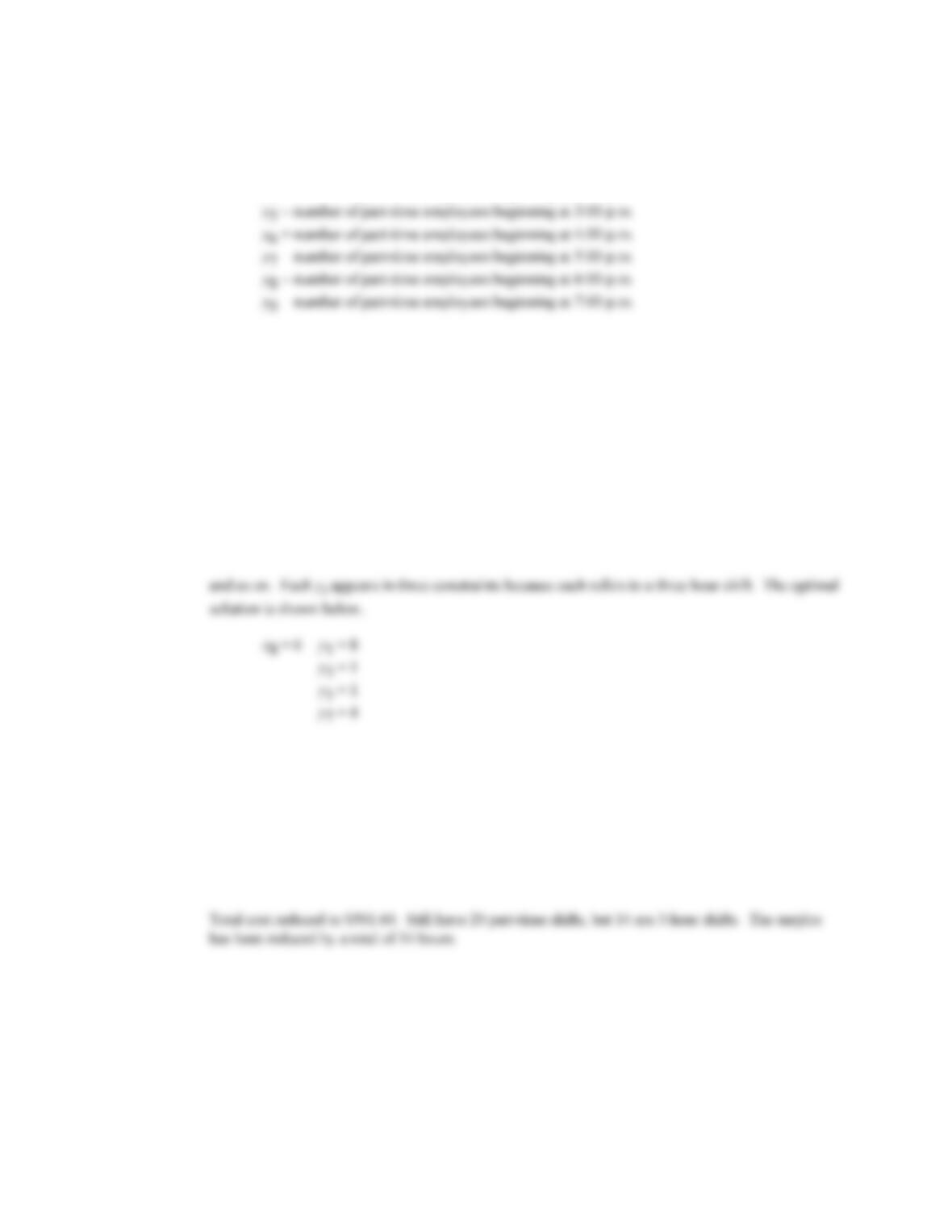
y1 = number of part-time employees beginning at 11:00 a.m.
y2 = number of part-time employees beginning at 12:00 p.m.
y3 = number of part-time employees beginning at 1:00 p.m.
y4 = number of part-time employees beginning at 2:00 p.m.
Each part-time employee assigned to a three-hour shift will be paid $7.60 (3 hours) = $22.80
New objective function:
89
11
min 30.40 22.80
ji
ji
xy
==
+
Each constraint must be modified with the addition of the yi variables. For instance, the first
constraint becomes
x1 + y1 8
Optimal schedule for part-time employees:
4-Hour Shifts
3-Hour Shifts
x8 = 6
y1 = 8
y3 = 1
y5 = 1
y7 = 4
Markov Processes
9 – 25