Chapter 08S – The Transportation Model
8S-1
CHAPTER 8S
THE TRANSPORTATION MODEL
Teaching Notes
The transportation method seems to be middle-of-the-road in terms of students’ abilities to develop an
intuitive feel for what is happening during the process. Although in practice much of the actual
computations are done by computers using the simplex algorithm, I feel that students gain a certain
amount of insight and intuitive understanding by going through the calculations.
Solutions to Problems
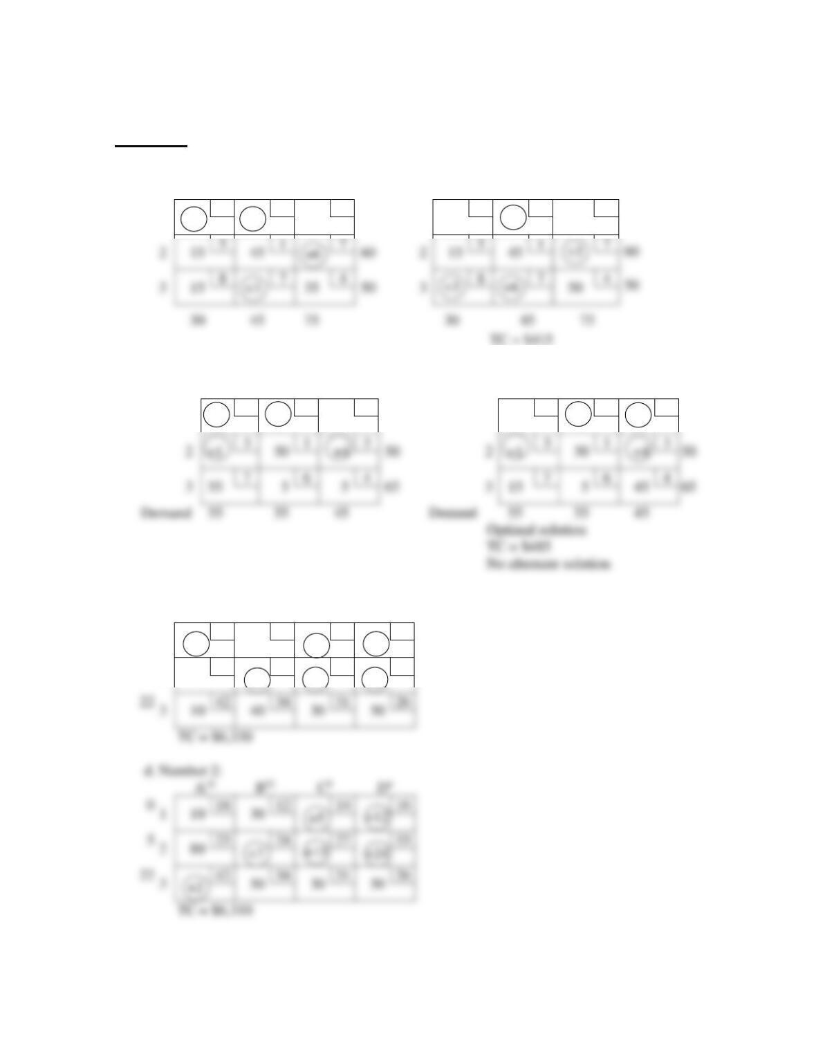
1. Ship 15 units from source 1 to destination 2
Ship 75 units from source 1 to destination 3
2. If N1 is opened, then the shipment schedule is as follows:
Ship 500 units from warehouse 1 to store B at a cost of $1,500
Ship 400 units from warehouse 2 to store A at a cost of $2,000
Chapter 08S – The Transportation Model
8S-2
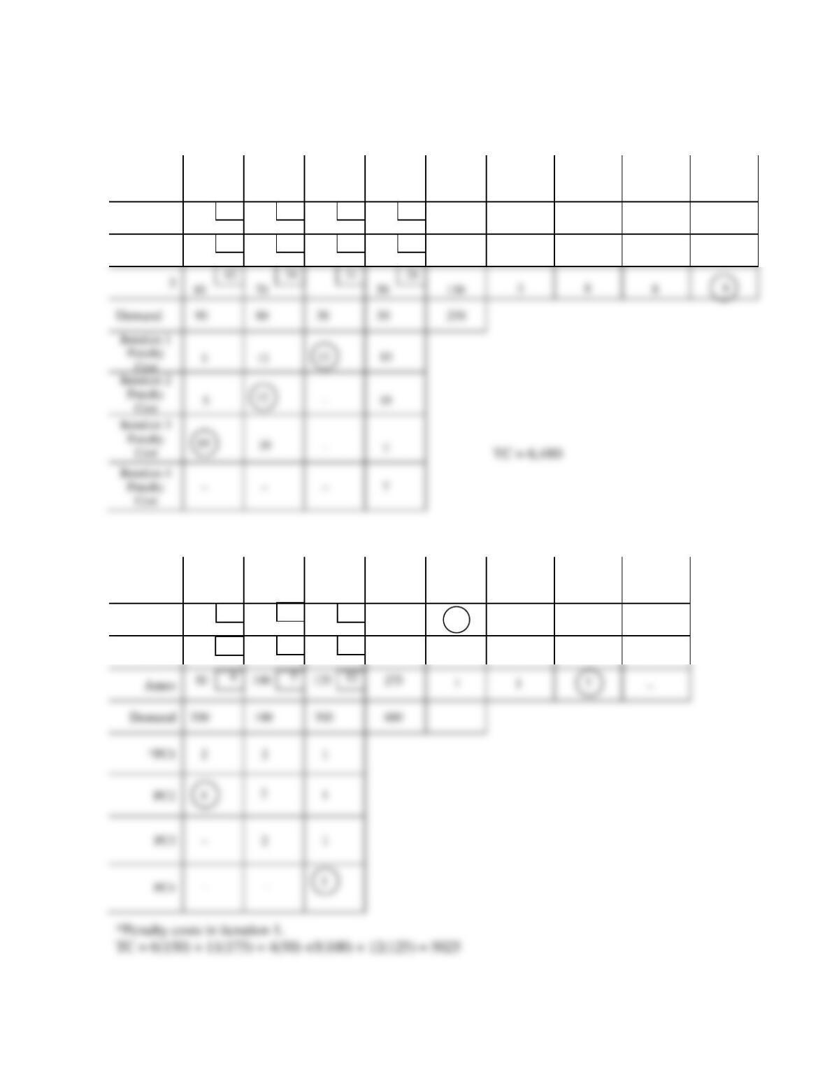
3. If the plant is located in Toledo, the shipment schedule is as follows:
Ship 210 units from Plant 1 to Destination C at a cost of $2,100
Ship 140 units from plant 2 to destination A at a cost of $1,680
Ship 80 units from plant 3 to destination A at a cost of $880
If the plant is located in Cincinnati, the shipment schedule is as follows:
Ship 210 units from plant 1 to destination C at a cost of $2,100
Ship 60 units from plant 2 to destination A at a cost of $720
Since 6,720 < 6,960, construct the new plant in Toledo.
4. If the store is opened in South Coast Plaza (SCP), then the shipment schedule and the related
costs are as follows:
Ship 500 units from warehouse 1 to store B at a cost of $4,500
Ship 160 units from warehouse 1 to SCP store at a cost of $640
Chapter 08S – The Transportation Model
If the store is opened in Fashion Island (FI), then the shipment schedule is as follows:
Ship 60 units from warehouse 1 to store A at a cost of $900
Ship 500 units from warehouse 1 to store B at a cost of $4,500
If the store is opened in Laguna Hill (LH), then the shipment schedule and the related costs are
as follows:
Ship 500 units from warehouse 1 to store B at a cost of $4,500
Ship 160 units from warehouse 1 to LH store at a cost of $800
Since 10,080 < 10,380 <10,500 open the store in South Coast Plaza.
“Advanced Topics: The Transportation Model” on the text web site
Answers to Discussion and Review Questions
2. Check to see that supply and demand are equal. If they are not, add a dummy origin or
3. No, a dummy is added to supply or demand, whichever is lower.
5. To maintain row and column totals.
7. The solution is not optimum.
8. a. Shift into the cell with the largest negative cell evaluation.
b. Identify the cell path used to evaluate that empty cell.
Chapter 08S – The Transportation Model
8S-4
10. The transportation method can be used to compare the total cost of alternative locations in
11. Total cost is the sum of the product of quantity and cell cost for all completed cells.
12. Quantities in dummy destinations indicate which origin will hold (not ship or not produce) the
13. The MODI method is a way to determine if a solution to a transportation problem is optimal.
It differs from the stepping-stone approach in that evaluation paths are not used. Instead, a set
of row and column index numbers are obtained. Both approaches yield the same results.
Chapter 08S – The Transportation Model
8S-5
Solutions
1.
Intuitive Solution: Intuitive rule
Number 2:
A
B
C
A
B
C
1
3
4
40
2
40
1
15
3
4
25
2
2. Solution
Number 2:
To:
1
2
3
Supply
To:
1
2
3
Supply
From:
1
–2
3
+2
6
40
2
40
From:
1
40
3
+4
6
+2
2
40
2
3
50
1
3
50
3
50
1
3
50
3
55
7
6
4
65
3
15
7
6
45
4
65
Demand
55
3. a,b,c Initial (Intuitive):
A20
B12
C9
D4
0
1
18
40
12
14
16
3
2
80
23
24
27
33
3
10
42
40
34
30
31
50
26
TC = $6,330
d. Number 2:
0
1
10
18
30
12
14
16
5
2
80
23
24
27
33
22
3
42
50
34
30
31
50
26
TC = $6,310
+5
+24
+13
+7
+2
–3
+2
+5
–2
+9
+15
+5
+12
+26
40
2
15
5
45
1
7
60
15
5
45
1
7
3
15
8
7
35
4
50
8
7
50
4
+3
+6
+3
+3
+6
Chapter 08S – The Transportation Model
8S-6
Solutions (continued)
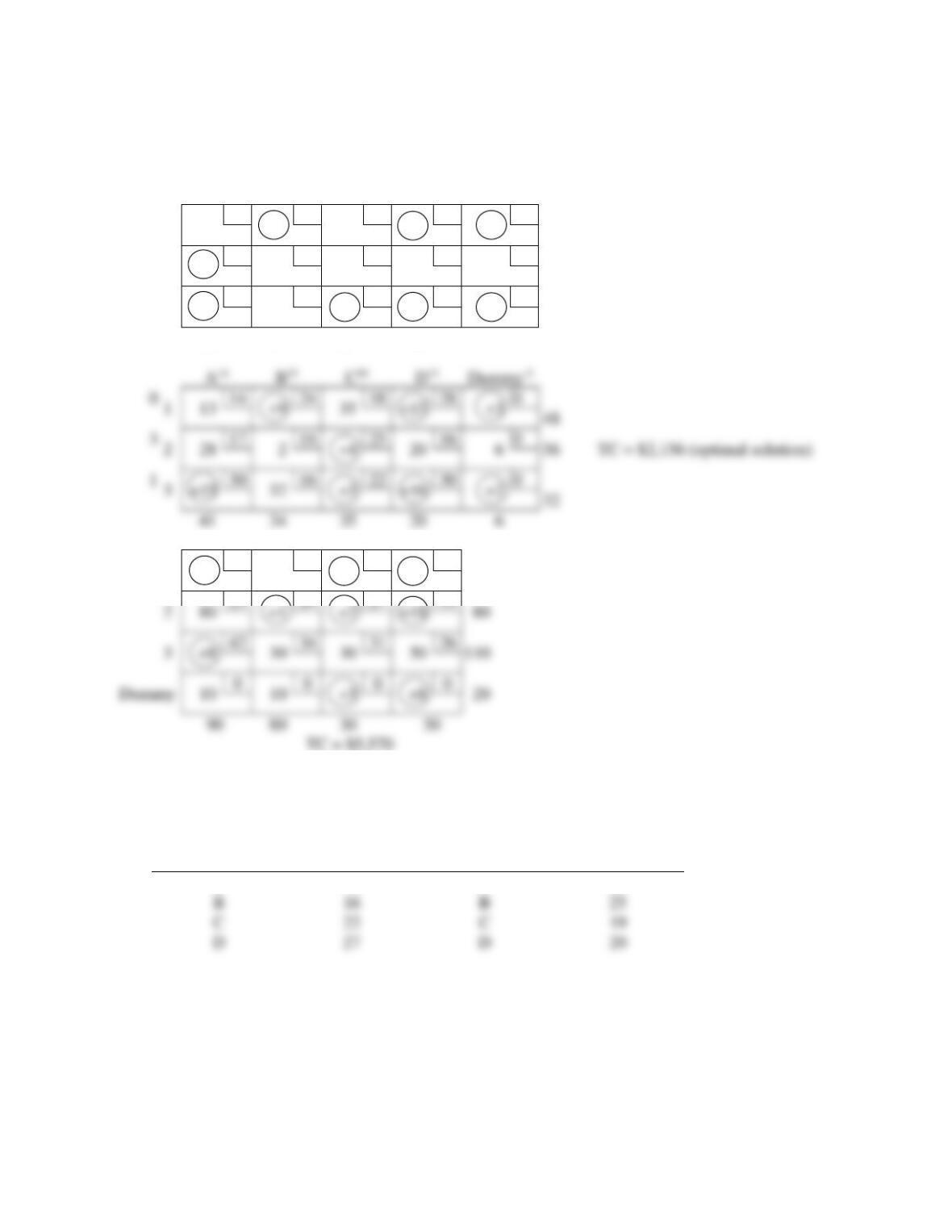
4.
Initial (Intuitive):
A14
B11
C18
D9
Dummy-7
0
1
41
14
+13
24
7
18
+19
28
+7
0
48
7
2
–4
17
2
18
28
25
20
16
6
0
56
5
3
+11
30
32
16
–1
22
+16
30
+2
0
32
41
34
35
20
6
5.
1
+6
18
40
12
+5
14
+12
16
40
2
80
23
+1
24
+7
27
+18
33
80
3
+8
42
30
34
30
31
50
26
110
Dummy
10
10
+3
+8
20
50
6. Instructors: Please let your students know that in answering this question, to use the following
table in lieu of the table given in problem 6.
From
Baltimore to
Cost per unit
From
Philadelphia to
Cost per unit
A
18
A
31
C
22
C
19
D
27
D
20
TC = $2,268
0
14
24
18
28
0
48
3
2
28
17
2
18
+4
25
20
16
6
0
TC = $2,156 (optimal solution)
1
3
+15
30
32
16
+3
22
+16
30
+2
0
32
Chapter 08S – The Transportation Model
8S-7
Solutions (continued)
Baltimore:
A14
B13
C18
D23
Dummy-4
0
1
41
14
+12
24
7
18
+5
28
+4
0
48
–7
2
+10
17
+12
18
+14
25
58
16
+11
0
58
TC = $2,842
4
3
+12
30
32
16
0
22
+3
30
0
0
32
4
Bal.
0
18
2
16
28
22
4
27
16
0
50
41
34
35
60
16
Philadelphia:
1
14
24
7
18
28
+1
0
48
2
17
2
18
25
54
16
+4
0
56
TC = $2,764
3
30
32
16
22
30
+6
0
32
Phil.
31
25
28
19
6
20
16
0
50
41
34
35
60
Chapter 08S – The Transportation Model
8S-8
Solutions (continued)
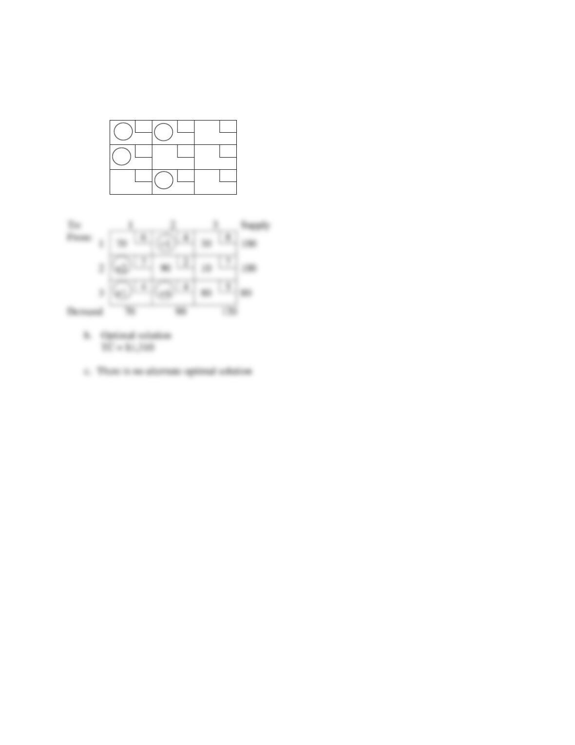
7. a. Solution
To:
1
2
3
Supply
From:
1
–1
6
+1
4
100
8
100
2
+1
7
90
2
10
7
100
3
70
4
+4
4
10
5
80
Demand
70
90
120
To:
1
2
3
Supply
From:
1
6
+1
4
8
100
2
7
2
7
100
3
+1
4
+4
4
80
5
80
Demand
70
120
Chapter 08S – The Transportation Model
8S-9
Solutions (continued)
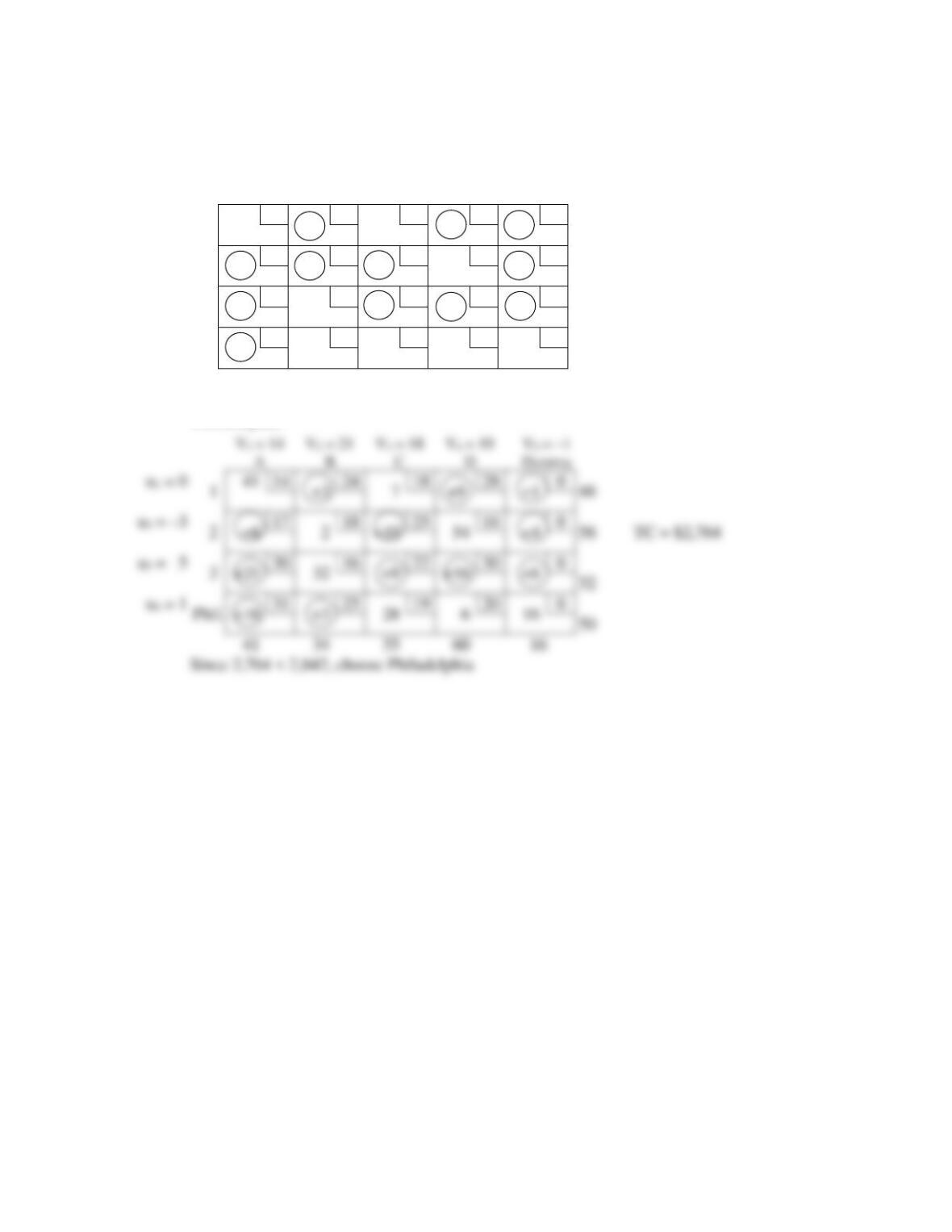
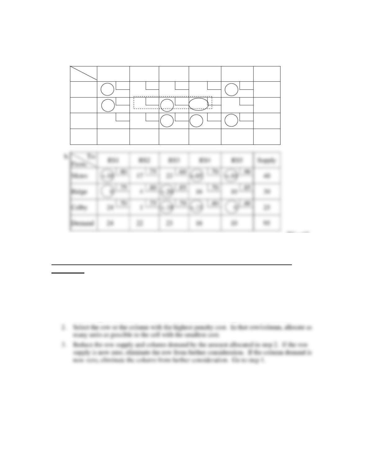
8. Initial (intuitive) solution is optional:
a.
To:
From:
RS1
RS2
RS3
RS4
RS5
Supply
Metro
+.10
.80
1
.75
23
.60
16
.70
+.10
.90
40
Ridge
0
.75
20
.80
+.20
.85
−0.05
.70
10
.85
30
Colby
24
.70
1
.75
+.10
.70
+.10
.80
0
.80
25
Demand
24
22
23
16
10
95
TC = 67
c. If Ridge-RS4 is not acceptable, the additional cost is 67.8 – 67 = .8 or $800.
Enrichment Module: Vogel’s Approximation Method and Supplemental
Problems
In addition to Intuitive Lowest-cost Approach, we can use Vogel’s Approximation to obtain an initial
reasonable solution.
Steps of Vogel’s Approximation
1. Determine the penalty cost for each row and each column. (Penalty cost is obtained by
subtracting the smallest cost from the next smallest cost in a given row or column).
(+)
(-)
(-)
(+)
To:
From:
RS1
RS2
RS3
RS4
RS5
Supply
Metro
+.10
.80
17
23
.60
+.05
.70
+.10
.90
40
Ridge
0
.75
4
+.20
.85
.70
10
.85
30
Colby
24
.70
1
+.10
.70
+.15
.80
0
.80
25
Demand
24
22
23
16
10
95
Chapter 08S – The Transportation Model
8S–10
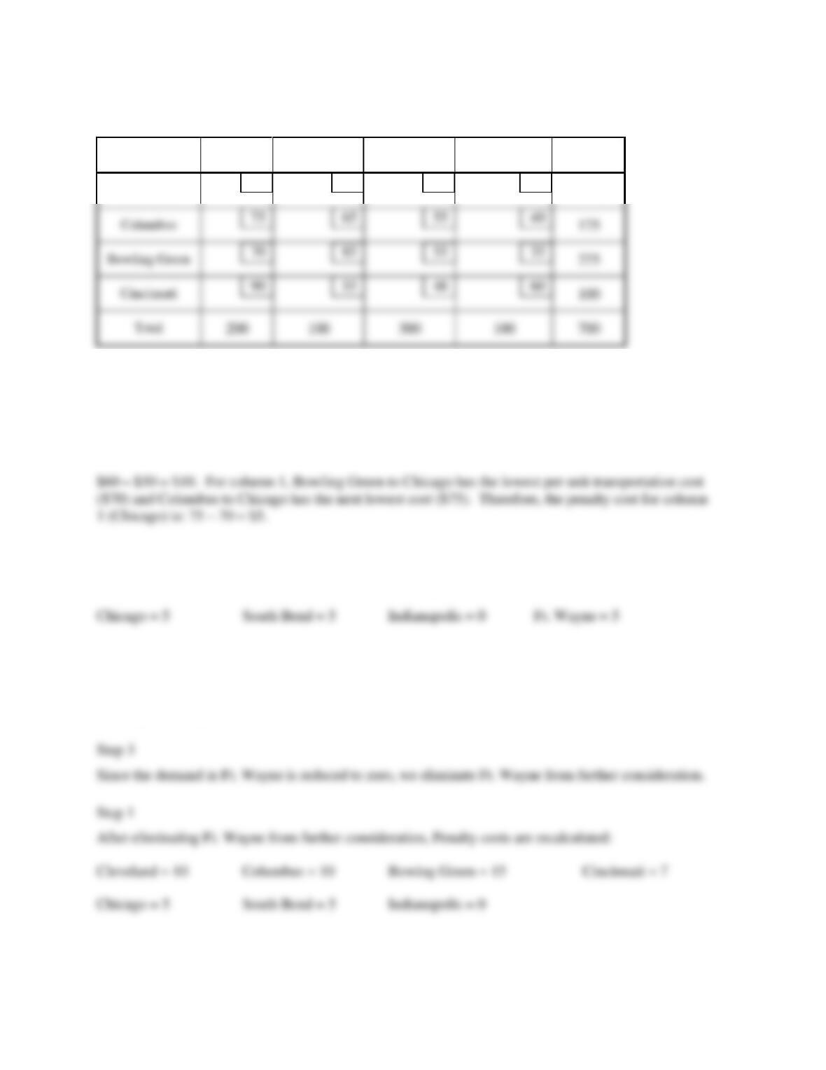
Example
TO
FROM
Chicago
South Bend
Indianapolis
Fort Wayne
Total
Cleveland
80
60
70
50
150
Step 1
In establishing the penalty cost for row 1 (Cleveland), we subtract the lowest cost in row 1 from the
second lowest cost in row 1. For Cleveland, the lowest cost is $50 (unit shipping cost from Cleveland
to Ft. Wayne). The second lowest cost is $60 (unit shipping cost from Cleveland to South Bend).
Proceeding in this fashion for the rest of the rows and columns, we obtain the following penalty costs:
Cleveland = 10 Columbus = 15 Bowling Green = 20 Cincinnati = 7
Step 2
Since row three (Bowling Green) has the largest penalty cost, it is selected. In row three, the shipping
route from Bowling Green to Ft. Wayne has the lowest shipping cost per unit ($35). Thus we allocate
as many units as possible (100 units) to it.
70
85
55
35
275
90
55
48
60
100
Chapter 08S – The Transportation Model
8S–11
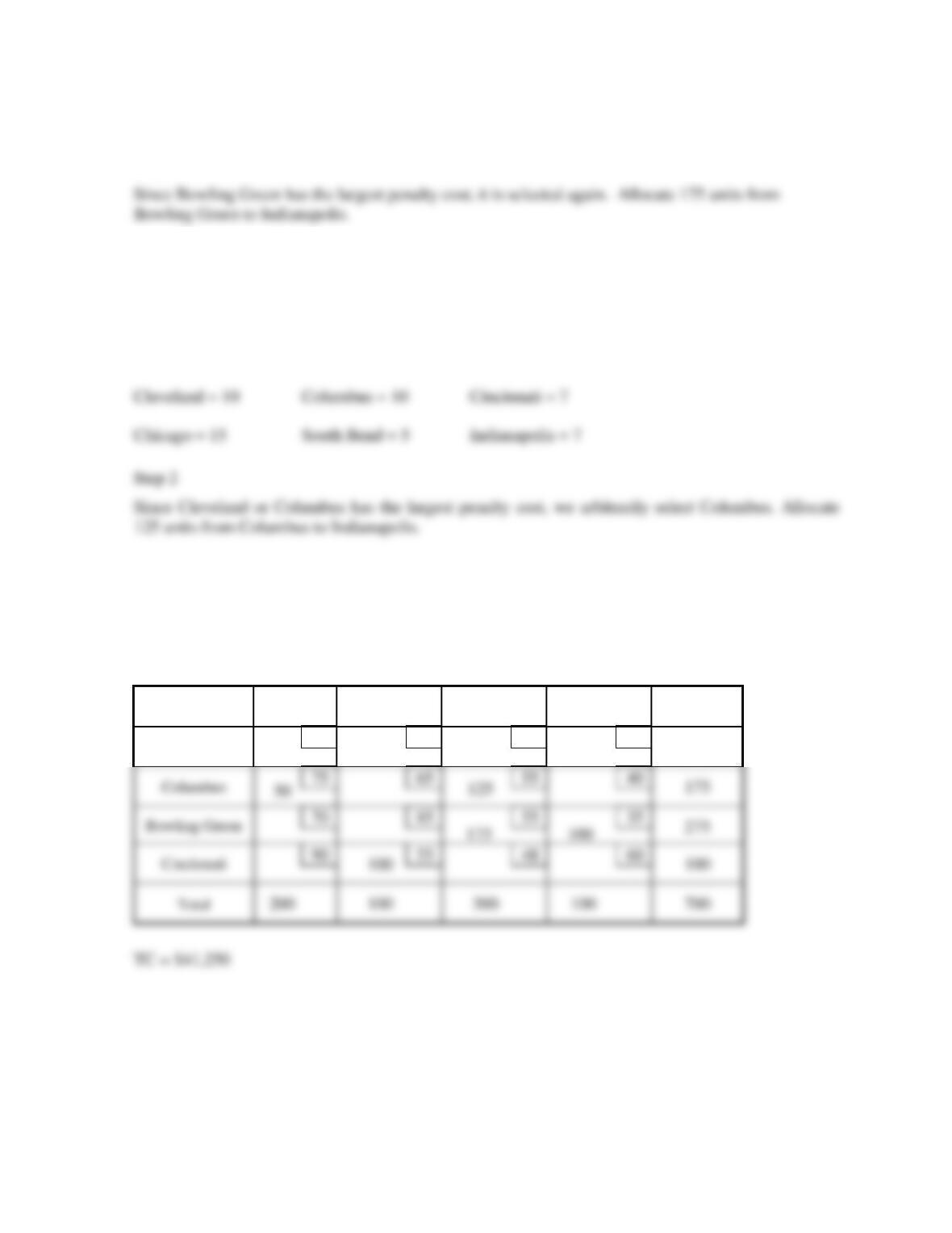
Step 2
Step 3
Eliminate Bowling Green from further consideration.
Step 1
Updated penalty costs are:
Step 3
Eliminate Indianapolis from further consideration.
Continuing in this fashion gives the following completed transportation table.
To
FROM
Chicago
South Bend
Indianapolis
Fort Wayne
Total
Cleveland
80
60
70
50
150
700
50
125
175
100
100
150
Chapter 08S – The Transportation Model
8S–12
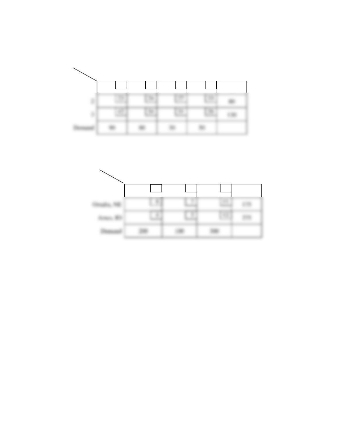
Exercise 1
For the following transportation tableau determine the initial feasible solution using Vogel’s
approximation.
To:
A
B
C
D
Supply
From
1
18
12
14
16
40
Exercise 2
For the following transportation tableau determine the initial feasible solution using Vogel’s
approxima-tion method.
To:
Milwaukee,
WI
St, Louis,
MO
Dayton,
OH
Supply
From
Wichita, KS
6
9
10
150
8
7
11
175
4
5
12
275
2
23
24
27
33
80
3
42
34
31
26
Chapter 08S – The Transportation Model
8S–13
Solution to Exercise 1 To
From
A
B
C
D
Supply
Iteration 1
Penalty
Cost
Iteration 2
Penalty
Cost
Iteration 3
Penalty
Cost
Iteration 4
Penalty
Cost
1
18
12
14
16
40
2
4
–
–
2
23
24
27
33
80
1
1
1
–
Solution to Exercise 2 To
MILW
SL
DAY
SUPPLY
PC1
PC2
PC3
PC4
Wichita
6
9
10
8
7
11
4
5
12
50
100
125
275
7
1
4
–
–
2
1
PC2
PC4
1
1
–
80
10
30
150
175
175
150
3
Omaha
–
–
–
1
1
4
–
3
42
34
31
26
10
70
50
7
–
–
5
5
5
8
8
Chapter 08S – The Transportation Model
8S–14
Supplemental Problems
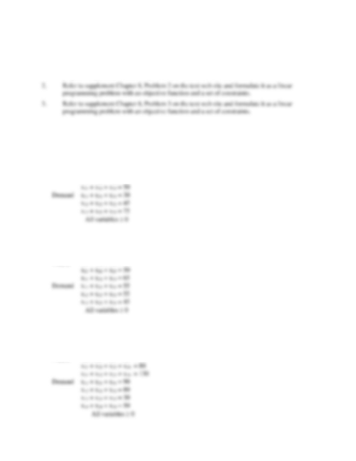
1. Refer to supplement Chapter 8, Problem 1 on the text web site and formulate it as a linear
programming problem with an objective function and a set of constraints.
Solutions to Supplemental Problems
1. x11 = quantity shipped from 1 to A, x12 = quantity shipped from 1 to B, etc.
Minimize Z = 3x11 + 4x12 + 2x13 + 5x21 + 1x22 + 7x23 + 8x31 + 7x32 + 4x33
s.t.
Supply x11 + x12 + x13 = 40
x21 + x22 + x23 = 60
2. x11 = quantity shipped from source 1 to destination 1, etc.
Minimize = 3x11 + 6x12 + 2x13 + 3x21 + x22 + 3x23 + 7x31 + 6x32 + 4x33
s.t.
Supply x11 + x12 + x13 = 40
3. x11 = quantity shipped from 1 to A, x12 = quantity shipped from 1 to B, etc.
Minimize Z = 18x11 + 12x12 + 14x13 + 16x14 + 23x21 + … + 26x34
s.t.
Supply x11 +x12 + x13 + x14 = 40