Performance – for Ch 8.xls, Instructions, page 1
Steady State Queuing Models 26 Oct 2007
John O. McClain jom1@cornell.edu
Johnson Graduate School of Management
Sage Hall, Cornell University
Ithaca NY 14853
This spreadsheet is intended for teaching purposes. You are welcome to use it in any
manner and change it as you see fit. This model comes without any guarantee, and is
distributed free of charge.
Note: If the worksheets don’t seem to work properly,
Click Here
Contents: Descriptions Models
The Models
The Finite Queue model assumes that there is a limit to the waiting line, and that
customers will not join the queue when that limit is reached. Those customers are
permanently lost, but the arrival rate of future customers is not affected.
Assumptions: Identical Servers, Poisson arrivals, Exponential service times.
The Infinite Queue model assumes that there is no limit to the waiting line. That is,
Each of these models is described in more detail below, and examples are worked out.
Steady State, Defined.
These models give “Steady State” results. This has two important implications:
●
The probability distributions of arrivals and service times do not change with time.
9% of the time there will be no one waiting. But the 9% does not apply, for example, if
For example, you cannot model variations in the arrivals at different times of day.
Using the Models
Your inputs always go in the yellow cells, like this:
Please be careful with your time units. Two of the inputs are rates, and they must have the
Performance – for Ch 8.xls, Instructions, page 2
Finite Queues (limited waiting line capacity)
Assumptions: Identical Servers, Poisson arrivals, Exponential service times.
The model also assumes that arrivals cease when the queue is full. This is “balking”.
Your Inputs: The 4 basic inputs for the finite queuing model are c, K, Ri and Rp.
There are c identical servers, and the queue can hold K customers.
Therefore the system can hold up to K+c customers (K in queue and c in service).
The arrival rate of customers is Ri, and the service rate is Rp for each server.
Example:
City Clinic serves a population that requires an average of 45 visits per 8-hour day.
Solution:
a.
On the Finite Queue worksheet, put in c = 2, K = 0, Ri = 45 and Rp = 25.
Go to the Finite Queue Graph sheet to see the entire probability distribution displayed.
c. Put in K=20 and Q=10. Answer: 19.22%
Experiments:
d. Using K=20 as the capacity of the waiting area, change the number of servers to 3
and watch what happens to the Finite Queue Graph.
Change the number of servers to 1 and watch what happens to the Finite Queue Graph.
Performance – for Ch 8.xls, Instructions, page 3
Infinite Queues (unlimited waiting line capacity)
Assumptions: Identical Servers, Poisson arrivals, Exponential service times.
Your Inputs: The 3 basic inputs for the infinite queuing model are c, K, Ri and Rp.
There are c identical servers, and the queue can hold an unlimited number of customers.
Example:
City Clinic serves a population that requires an average of 45 visits per 8-hour day.
There are two nurse-practitioners, each capable of serving 25 patients per day.
e. Does the use of a priority system change the total size of the waiting line?
Solution:
a.
On the Infinite Queue worksheet, put in c = 2, Ri = 45 and Rp = 25.
This will cause Ii = 7.674 patients waiting, on average, and Ti = 0.1705 days waiting,
Performance – for Ch 8.xls, Infinite Queue, page 4
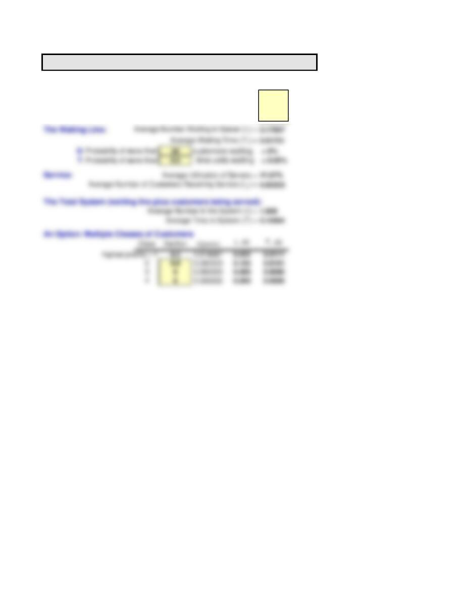
Steady-State, Infinite Capacity Queues
Basic Inputs: Number of Servers, c =2
Arrival Rate, Ri = 10
Service Rate of each server, 1/Tp =12
Model is OK
Performance – for Ch 8.xls, Finite Queue, page 5
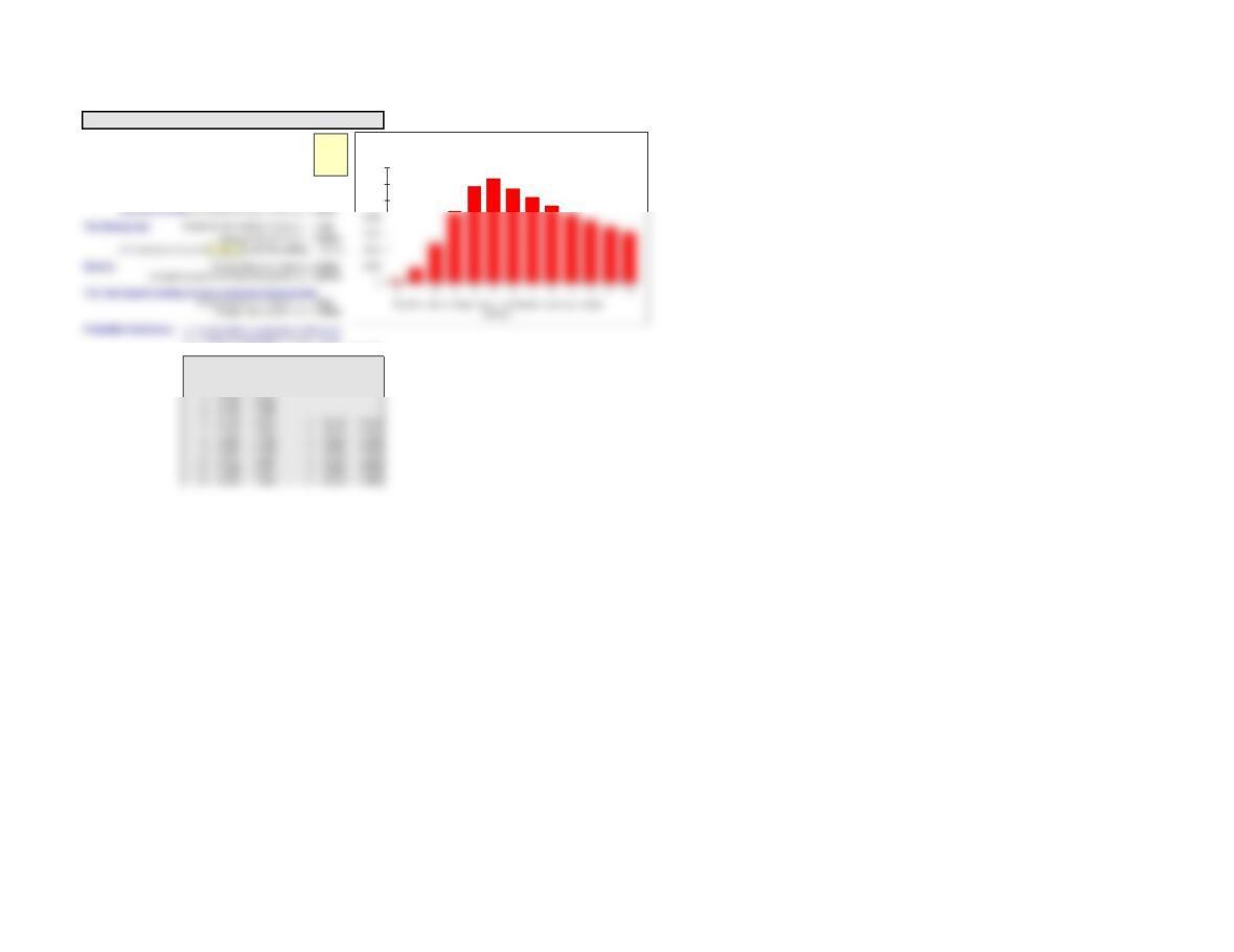
Steady-State, Finite Capacity Queues 6 Servers, Queue Capacity = 6, Arrival Rate = 5, Service Rate = 0.923076923076923
Basic Inputs: Number of Servers, c = 6
Queue Capacity, K =6
Arrival Rate, Ri =5
Service Rate Capacity of each server, Rp =0.92308
Arrivals:
Average Rate Joining System (R) = 4.69048
Average Rate Leaving Without Service (RiPb) = 0.30952
n P(n) Cumulative q P(q) Cumulative
0 0.0033 0.0033
1 0.0177 0.0209
2 0.0478 0.0687
3 0.0863 0.1551
0.1
0.12
0.14
Steady-State Probabilities for Finite Capacity Queue
6 Servers, Queue Capacity = 6, Arrival Rate = 5, Service Rate = 0.923076923076923