8 –
1
Chapter 8
Linear Programming: Sensitivity Analysis and Interpretation of
Solution
Case Problem 1: Product Mix
Note to Instructor: The difference between relevant and sunk costs is critical. The cost of the shipment of nuts is a
sunk cost. Practice in applying sensitivity analysis to a business decision is obtained. You may want to suggest that
sensitivity analyses other than the ones we have suggested be undertaken.
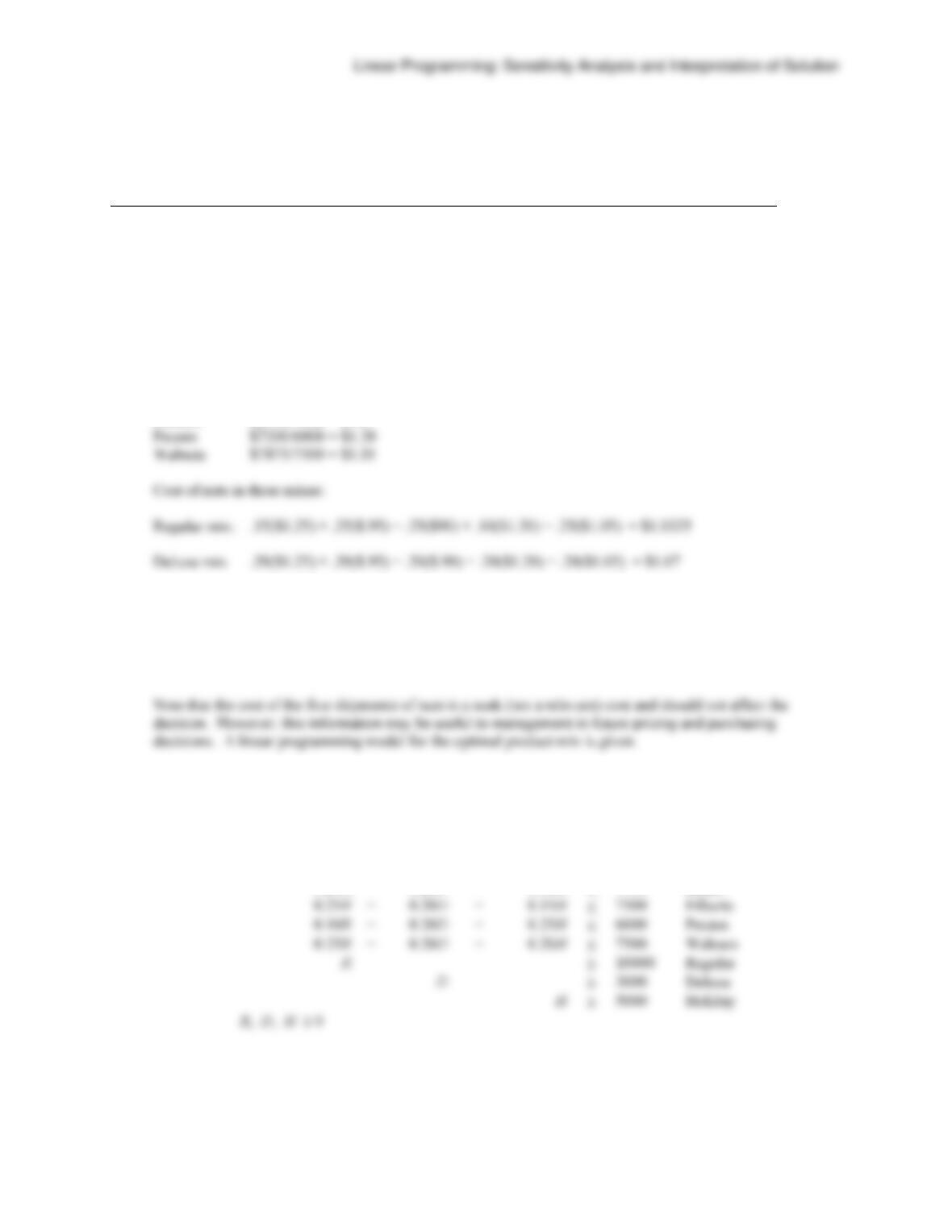
1. Cost per pound of ingredients
Almonds $7500/6000 = $1.25
Brazil $7125/7500 = $.95
Holiday mix: .25($1.25) + .15($.95) + .15($.90) + .25($1.20) + .20($1.05) = $1.10
2. Let R = pounds of Regular Mix produced
D = pounds of Deluxe Mix produced
H = pounds of Holiday Mix produced
The following linear programming model can be solved to maximize profit contribution for the nuts already
purchased.
Max
1.65R
+
2.00D
+
2.25H
s.t.
0.15R
+
0.20D
+
0.25H
6000
Almonds
0.25R
+
0.20D
+
0.20H
7500
Walnuts
10000
Regular
Chapter 8
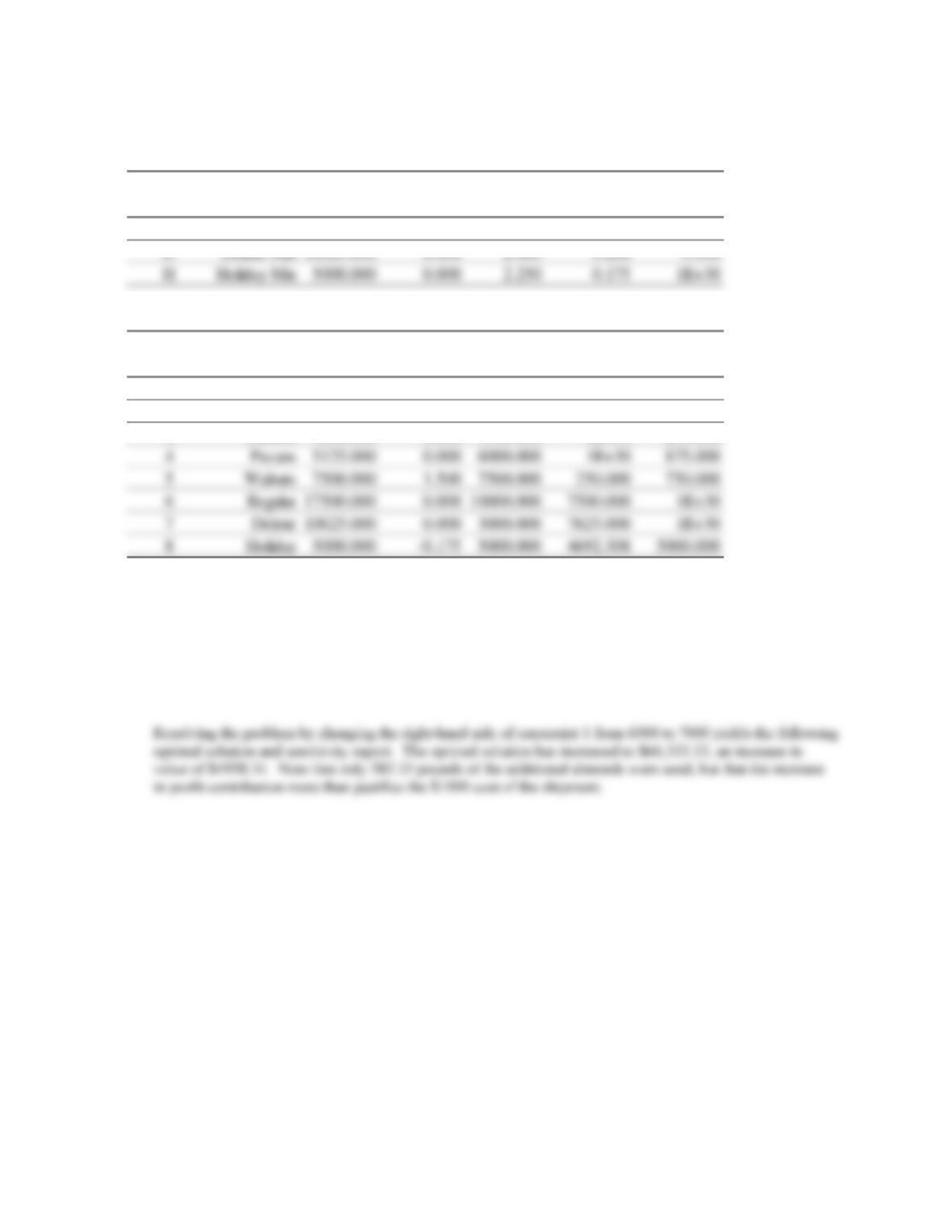
The sensitivity report for this problem is shown below. The optimal objective function value is $61,375.00.
Variable Cells
Model Final Reduced Objective Allowable Allowable
Variable Name Value Cost
Coefficient
Increase Decrease
R Reular Mix 17500.000 0.000 1.650 0.350 0.150
Constraints
Constraint Final Shadow Constraint Allowable Allowable
Number Name Value Price R.H. Side Increase Decrease
1 Almonds 6000.000 8.500 6000.000 583.333 610.000
2 Brazil 7250.000 0.000 7500.000 1E+30 250.000
3. From the shadow prices it can be seen that additional almonds are worth $8.50 per pound to TJ. Additional
walnuts are worth $1.50 per pound. From the slack values, we see that additional Brazil nut, Filberts, and
Pecans are of no value since they are already in excess supply.
4. Yes, purchase the almonds. The shadow price shows that each pound is worth $8.50; the shadow price is
applicable for increases up to 583.33 pounds.
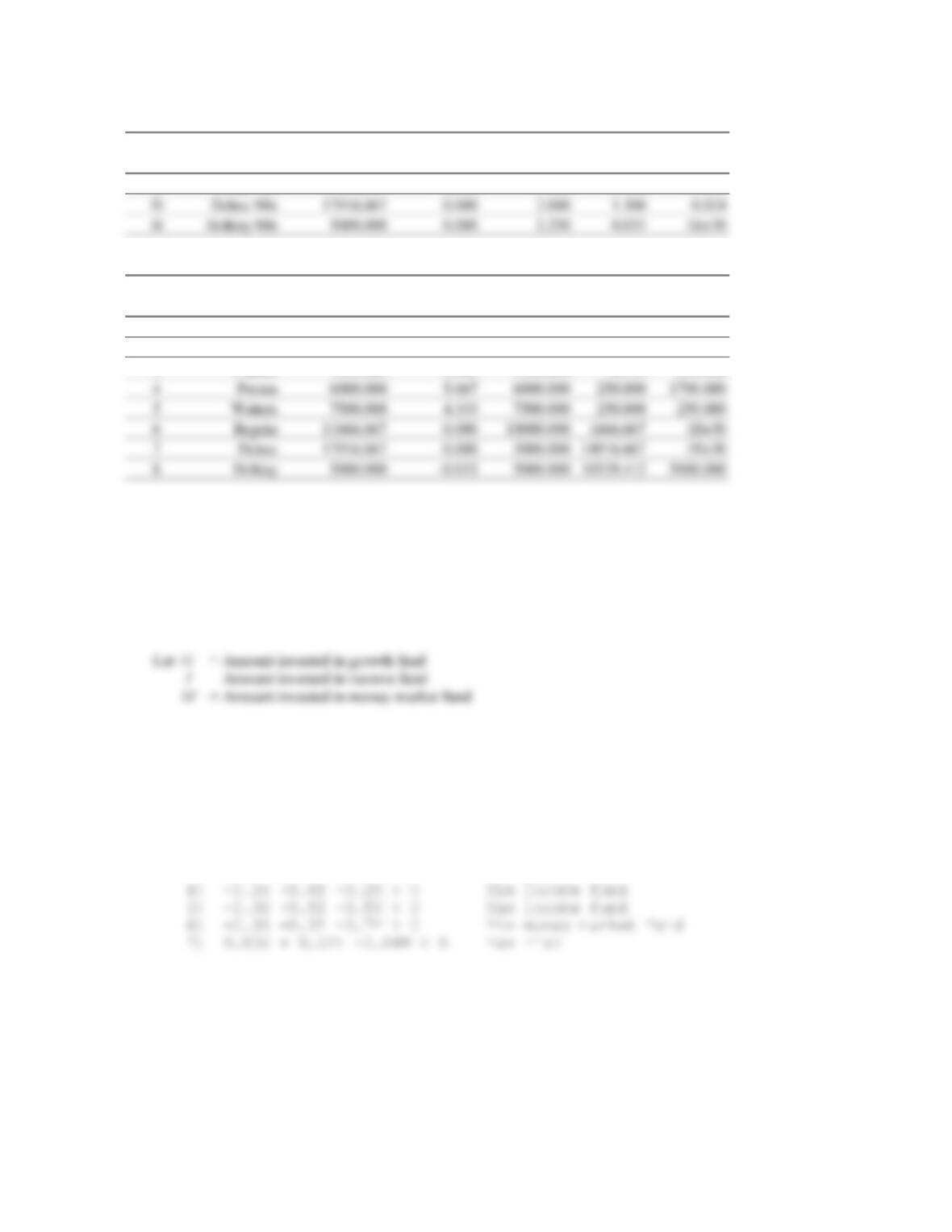
Variable Cells
Model Final Reduced Objective Allowable Allowable
Variable Name Value Cost Coefficient Increase Decrease
R Reular Mix 11666.667 0.000 1.650 0.100 0.650
Constraints
Constraint Final Shadow Constraint Allowable Allowable
Number Name Value Price R.H. Side Increase Decrease
1 Almonds 6583.333 0.000 7000.000 1E+30 416.667
2 Brazil 7250.000 0.000 7500.000 1E+30 250.000
5. From the shadow prices it is clear that there is no advantage to not satisfying the orders for the Regular and
Deluxe mixes. However, it would be advantageous to negotiate a decrease in the Holiday mix requirement.
Case Problem 2: Investment Strategy
1. The first step is to develop a linear programming model for maximizing return subject to constraints for funds
available, diversity, and risk tolerance.
The LP formulation is shown below.
MAX 0.18G + 0.125I + 0.075M
S.T.
1) G + I + M < 800000 Funds Available
2) 0.8G –0.2I –0.2M > 0 Min growth fund
3) 0.6G –0.4I –0.4M < 0 Max growth fund
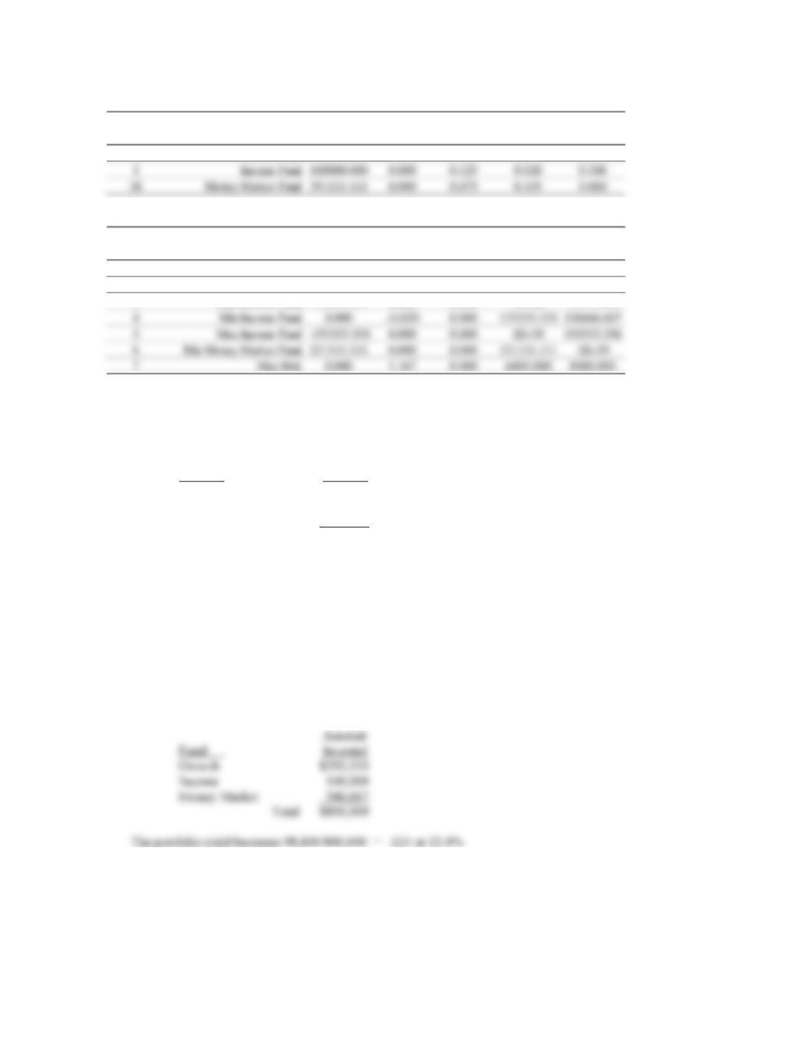
The optimal objective function value is 94,133.336. The sensitivity report for the optimal solution to this problem is:
Chapter 8
Variable Cells
Model Final Reduced Objective Allowable Allowable
Variable Name Value Cost Coefficient Increase Decrease
G Growth Fund 248888.889 0.000 0.180 1E+30 0.030
Constraints
Constraint Final Shadow Constraint Allowable Allowable
Number Name Value Price R.H. Side Increase Decrease
1 Funds Available 800000.000 0.118 800000.000 1E+30 800000.000
2 Min Growth Fund 88888.889 0.000 0.000 88888.889 1E+30
Rounding to the nearest dollar, the portfolio recommendation for Langford is as follows.
Amount
Fund: Invested
Growth $248,889
Income 160,000
Money Market 391,111
Total $800,000
Yield = 94,133 / 800,000 = .118
The portfolio yield is .118 or 11.8%.
Note that the portfolio yield equals the shadow price for the funds available constraint.
2. If Langford’s risk index is increased by .005 that is the same as increasing the right-hand side of constraint 7
by .005 (800,000) = 4000. Since this amount of increase is within the right-hand-side range, we would
expect an increase in return of 1.167 (4000) = 4668. The revised formulation and new optimal solution are
shown below. Except for rounding, the value has increased as predicted; the new optimal allocation is
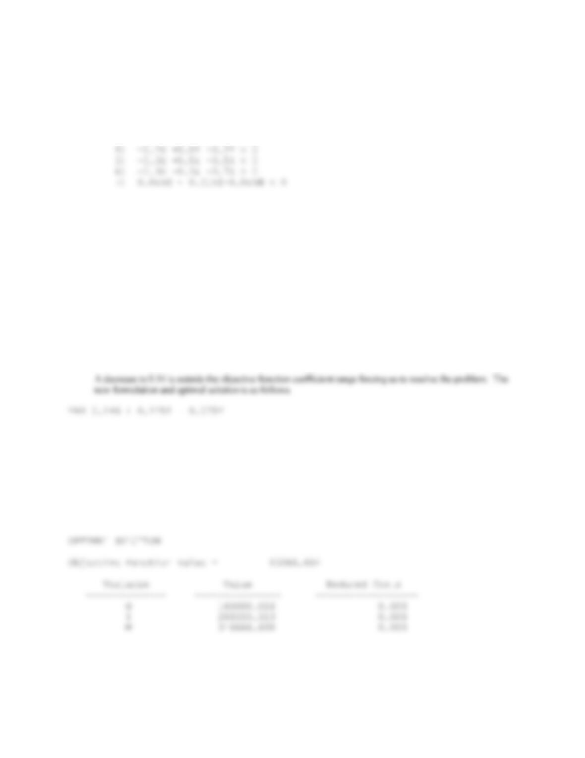
MAX 0.18G + 0.125I + 0.075M
S.T.
1) G + I + M < 800000
2) 0.8G –0.2I –0.2M > 0
3) 0.6G –0.4I –0.4M < 0
OPTIMAL SOLUTION
Objective Function Value = 98800.000
Variable Value Reduced Costs
————– ————— ——————
G 293333.313 0.000
I 160000.000 0.000
M 346666.656 0.000
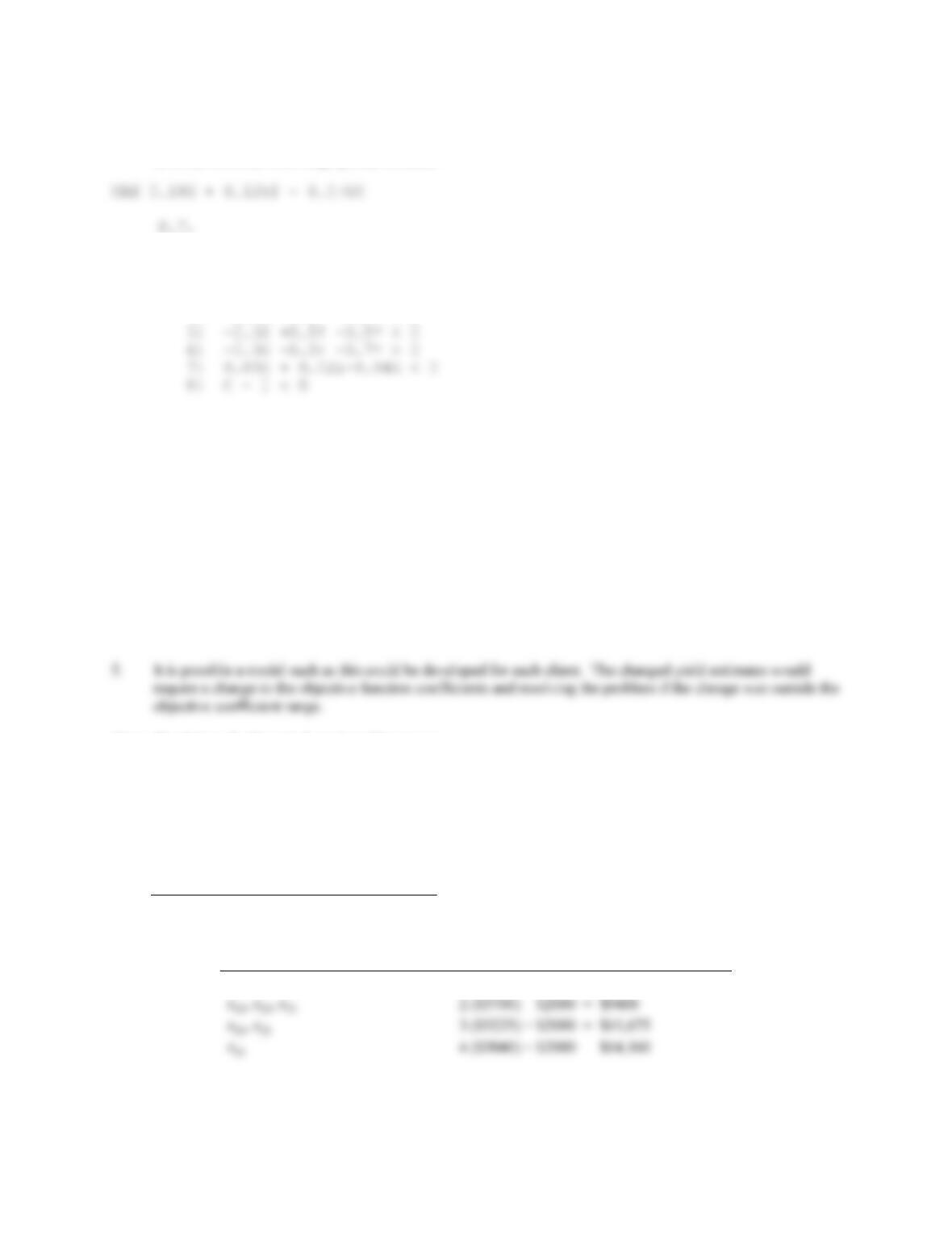
3. Since 0.16 is in the objective coefficient range for the growth fund return, there would be no change in
allocation. However, the return would decrease by (0.02) ($248,889) = $4978.
S.T.
1) G + I + M < 800000
2) 0.8G –0.2I –0.2M > 0
3) 0.6G –0.4I –0.4M < 0
4) –0.2G +0.8I –0.2M > 0
5) –0.5G +0.5I –0.5M < 0
6) –0.3G –0.3I +0.7M > 0
7) 0.05G + 0.02I–0.04M < 0
Chapter 8
4. Since the current optimal solution has more invested in the growth fund than the income fund, adding this
requirement will force us to resolve the problem with a new constraint. We should expect a decrease in return
as is shown in the following optimal solution.
1) G + I + M < 800000
2) 0.8G –0.2I –0.2M > 0
3) 0.6G –0.4I –0.4M < 0
4) –0.2G +0.8I –0.2M > 0
OPTIMAL SOLUTION
Objective Function Value = 93066.656
Variable Value Reduced Costs
————– ————— ——————
G 213333.313 0.000
I 213333.313 0.000
M 373333.313 0.000
Note that the value of the solution has decreased from $94,133 to $93,067. This is only a decrease of 0.2%
inyield. Since the yield decrease is so small, Williams may prefer this portfolio for Langford.
Case Problem 3: Truck Leasing Strategy
1. Let
ij
x
= number of trucks obtained from a short term lease signed in month i for a period of j months
i
y
= number of trucks obtained from the long-term lease that are used in month i
Monthly fuel costs are 20 ($100) = $2000.
Monthly Costs for Short-Term Leased Trucks
Note: the costs shown here include monthly fuel costs of $2000.
Decision Variables
Cost
x11, x21, x31, x41
$4000 + $2000 = $6000
x12, x22, x32
2 ($3700) + $2000 = $9400
x13, x23
3 ($3225) + $2000 = $11,675
x14
4 ($3040) + $2000 = $14,160
Monthly Costs for Long-Term Leased Trucks
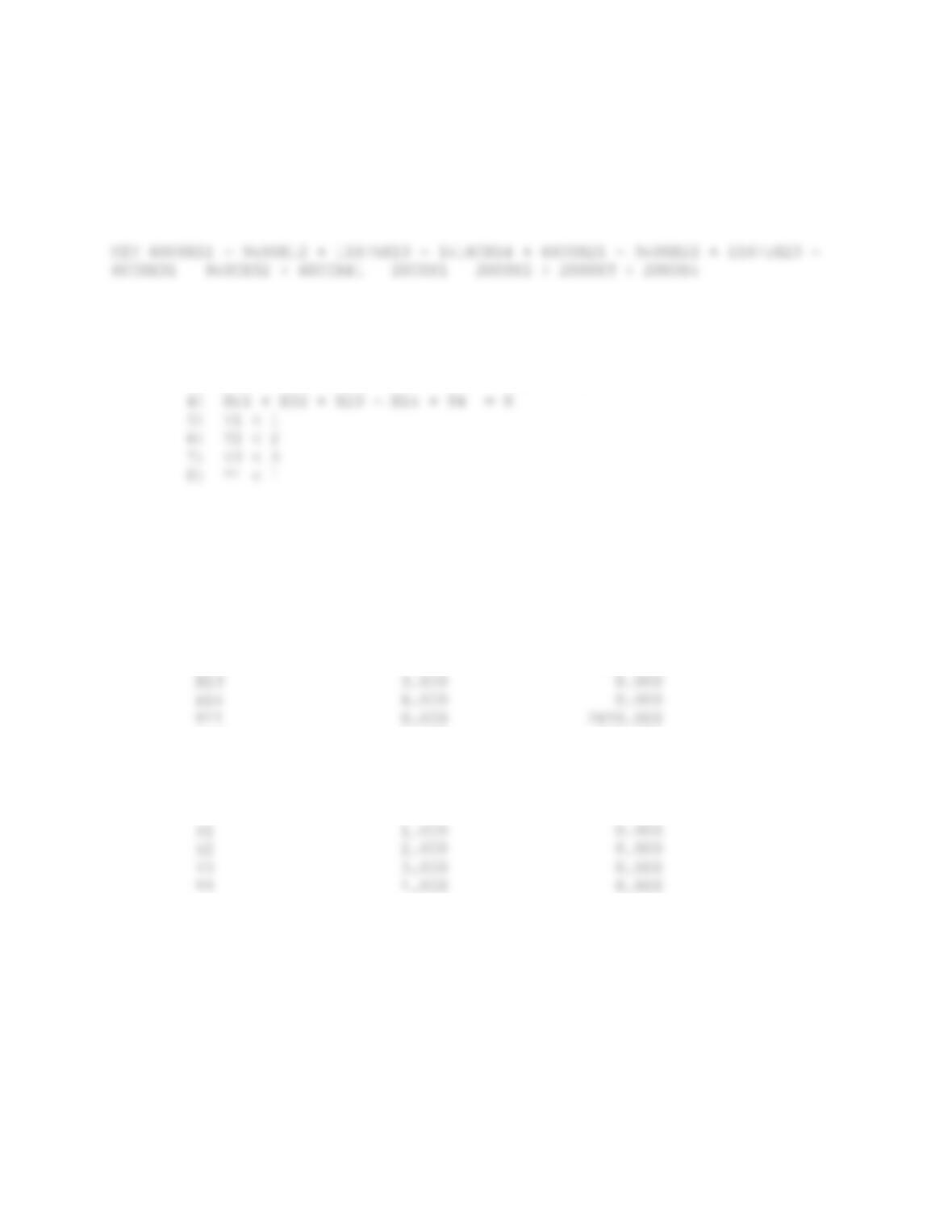
Since Reep Construction is committed to the long-term lease and since employees cannot be laid off, the
only relevant cost for the long-term leased trucks is the monthly fuel cost of $2000.
The model formulation for this problem is shown below.
S.T.
1) X11 + X12 + X13 + X14 + Y1 = 10
2) X21 + X22 + X23 + X14 + X13 + X12 + Y2 = 12
3) X31 + X32 + X23 + X22 + X14 + X13 + Y3 = 14
The optimal solution to this problem is:
Objective Function Value = 151660.000
Variable Value Reduced Costs
————– ————— ——————
X11 0.000 3515.000
X12 0.000 3725.000
X22 0.000 210.000
X23 1.000 0.000
X31 1.000 0.000
X32 0.000 915.000
X41 0.000 3515.000
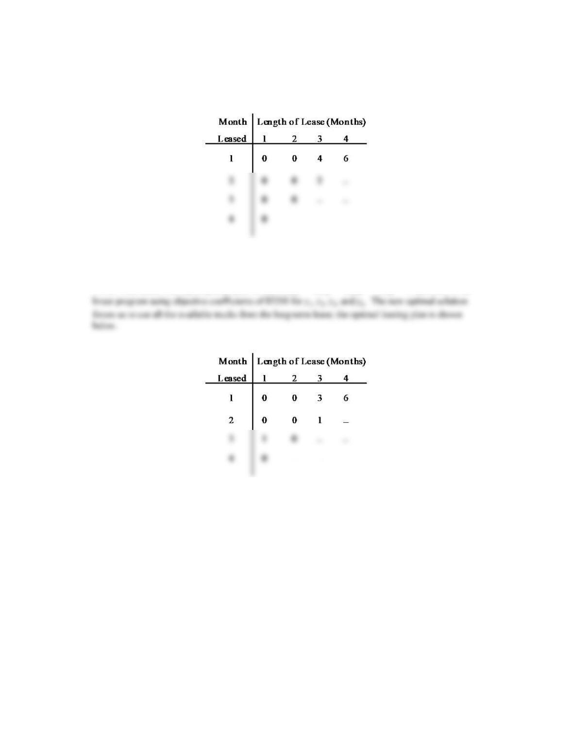
2. The total cost associated with the leasing plan is $151,660.
Chapter 8
3. If Reep Construction is willing to consider the possibility of layoffs, we need to include driver costs of
$3200 per month. Replacing the coefficients for y1, y2, y3, and y4 in our previous linear program with
$5200 and resolving resulted in the following leasing plan:
In addition, in month 3, two of the trucks from the long-term leases were used. The total cost of this leasing
plan is $165,410.
To see what effect a no layoff policy has, we can set y1 = 1, y2 = 2, y3 = 3, y4 = 1 and resolve the
The total cost associated with this solution is $174,060. Thus, if Reep maintains their current policy of no
layoffs they will incur an additional cost of $174,060 – $165,410 = $8,650.
Markov Processes
8 –
1