8 – 1
Chapter 8
Linear Programming: Sensitivity Analysis
and Interpretation of Solution
Learning Objectives
1. Understand what happens in graphical solutions when coefficients of the objective function change.
2. Be able to interpret the range for an objective function coefficient.
6. Understand the limitations of classical sensitivity analysis.
7. Learn how to formulate, solve and interpret the solution for linear programs with more than two
decision variables.
8. Understand the following terms:
Markov Processes
8 – 1
Solutions:
1. a.
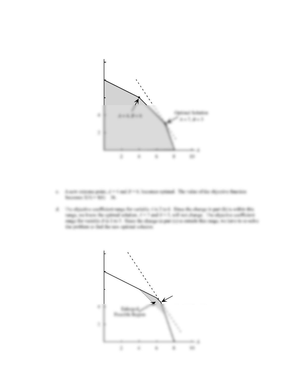
b. The same extreme point, A = 7 and B = 3, remains optimal.
The value of the objective function becomes 5(7) + 2(3) = 41
2. a.
B
6
8
10
3(7) + 2(3) = 27
B
Optimal Solution
6
8
10
A = 6.5, B = 4.5
3(6.5) + 2(4.5) = 28.5
Chapter 17
8 – 2
b. The value of the optimal solution to the revised problem is 3(6.5) + 2(4.5) = 28.5. The one-unit
increase in the right-hand side of constraint 1 has improved the value of the optimal solution by 28.5
– 27 = 1.5. Thus, the shadow price for constraint 1 is 1.5.
3. a.
b. The same extreme point, X = 3 and Y = 2, remains optimal.
The value of the objective function becomes 6(3) + 12(2) = 42.
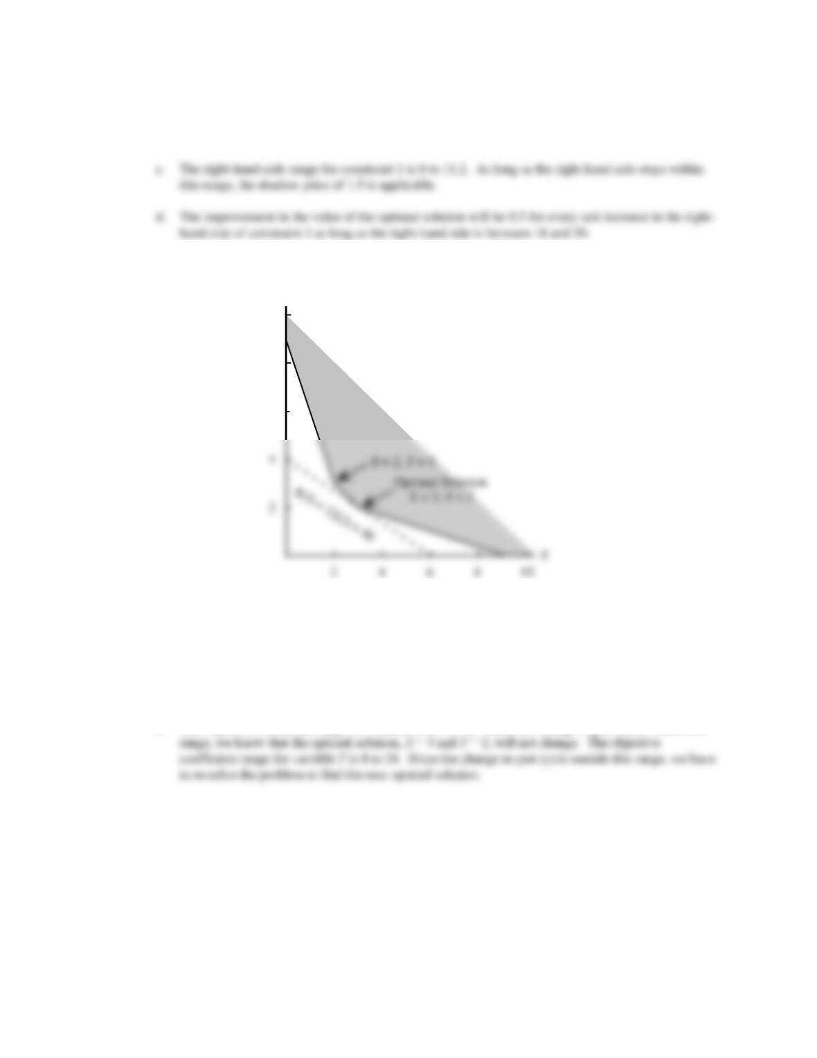
c. A new extreme point, X = 2 and Y = 3, becomes optimal. The value of the objective function
becomes 8(2) + 6(3) = 34.
d. The objective coefficient range for variable X is 4 to 12. Since the change in part (b) is within this
Y
6
8
10
Markov Processes
8 – 3
4. a.
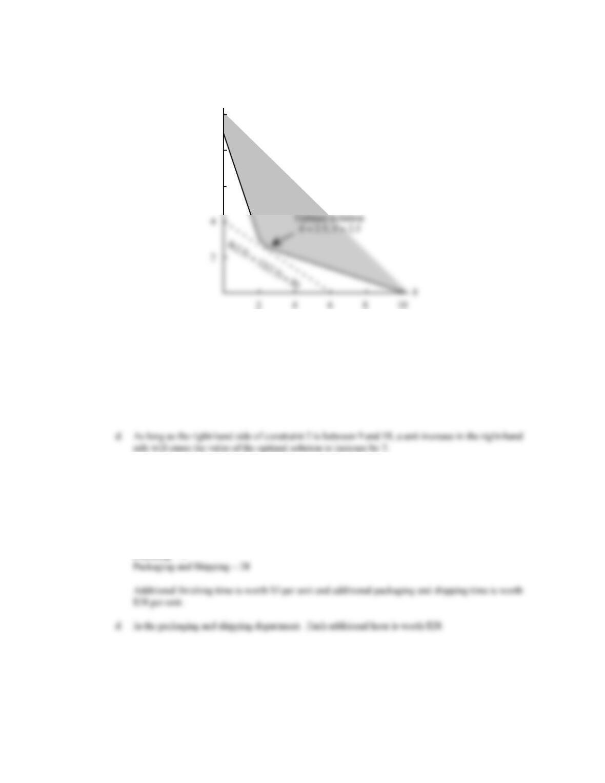
b. The value of the optimal solution to the revised problem is 8(2.5) + 12(2.5) = 50. Compared to the
original problem, the value of the optimal solution has increased by 50 – 48 = 2. However, this is a
minimization problem and the increase of 2 is not an improvement in the value of the optimal
solution. In fact, the value of the optimal solution is worse by 2. Thus, the shadow price is 2.
c. The right-hand side range for constraint 1 is 5 to 11. As long as the right-hand side stays within this
range, the shadow price of 2 is applicable. Since increasing the right-hand increases the value of the
optimal solution, decreasing the right-hand side of constraint 1 would b desirable.
5. a. Regular Glove = 500
Catcher’s Mitt = 150
Value = 5(500) + 8(150) = 3700
b. The finishing and packaging and shipping constraints are binding.
c. Cutting and Sewing = 0
Y
6
8
10
Chapter 17
8 – 4
6. a. The optimal value for the Regular Glove variable is 5, the Allowable Decrease is 1 and the
Allowable Increase is 7. The optimal value for the Catcher’s Mitt variable is 8, the Allowable
Decrease is 4.667 and the Allowable Increase is 2. Therefore, we can express the Objective
Coefficient Ranges as:
Variable
Objective Coefficient Range
Regular Glove
5–1 = 4 to 5+7 = 12
Catcher’s Mitt
8–4.667 = 3.333 to 8+2 = 10
c. The shadow prices for the resources are applicable over the following ranges:
Constraint
Right-Hand-Side Range
Cutting and Sewing
900-175 = 725 to No Upper Limit
Finishing
300-166.667 = 133.333 to 300+100 = 400
Packaging
100-25 = 75 to 100+35 = 135
d. The shadow price of packaging and shipping constraint is 28, so the amount of increase = (28) (20) =
$560
c.
Constraint
Shadow Price
Funds Avail.
0.093
Risk Max
1.333
U.S. Oil Max
0
d. No, the optimal solution does not call for investing the maximum amount in U.S. Oil.
8. a. The allowable increase for U.S. Oil is 7.000, so by more than $7.00 per share.
9. a. The optimal solution calls for the production of 560 jars of Western Foods Salsa and 240 jars of
Mexico City Salsa; profit is 1(560) + 1.25(240) = $860.
Markov Processes
8 – 5
b.
Variable
Objective Coefficient Range
Western Foods Salsa
1.000-0.107 = 0.893 to 1.000 + 0.250 = 1.250
c.
Constraint
Shadow
Price
Interpretation
1
0.125
One more ounce of whole tomatoes will increase profits by
$0.125
2
0.000
Additional ounces of tomato sauce will not improve profits;
0.188
One more ounce of tomato paste will increase profits by $0.188
d.
Constraint
Right-Hand-Side Range
Whole tomatoes
4480-160 = 4320 to 4480+1120
Tomato paste
1600-320 = 1280 to 1600+40 =
1640
10. a. S = 4000
M = 10,000
Total risk = 8(4000) + 3(10,000) = 62,000
b.
Variable
Objective Coefficient Range
S
8.000-4.250=3.750 to No
No Upper Limit to
e. 0.057 risk units
f. 0.057(100) = 5.7%
11. a. No change in optimal solution; the allowable increase for the objective coefficient for S is infinite.
b. No change in the optimal solution; the allowable increase for the objective coefficient for M is 3.400.
12. a. E = 80, S = 120, D = 0
Profit = 63(80) + 95(120) + 135(0) = $16,440
Chapter 17
8 – 6
b. The fan motors and cooling coils constraints are binding.
c. The manufacturing time constraint has slack; 2400-2080 = 320 hours are available.
13. a. The range of optimality for each objective function coefficient is as follows:
E 63.000 – 15.5000 = 47.500 to 63.000+12.000 = 75
S 95.000-8.000 = 87.000 to 95.000+31.000 = 126
D No lower limit to135.000+24.000 = 159.000
c. The range of feasibility for the right-hand side values for each constraint are as follows:
Fan motors constraint 200.000-40.000 = 160.000 to 200.000+80.000 = 280.000
Cooling coils constraint 320.000-120.000 = 200.000 to 320.000+80.000 = 400.000
Manufacturing time constraint 2400.000-320.000 = 2080.000 to No Upper Limit
d. Yes, 100 is greater than the allowable increase for the fan motors constraint (80.000).
The shadow price will change.
14. a. The optimal solution is to manufacture 100 cases of model A, 60 cases of model B and purchase 90
cases of model B
Total Cost = 10(100) + 6(60) + 14(0) + 9(90) = $2170
If demand for model A increases by 1 unit, total cost will increase by $12.25
If demand for model B increases by 1 unit, total cost will increase by $9.00
If an additional minute of assembly time is available, total cost will decrease by $.375
d. The assembly time constraint. Each additional minute of assembly time will decrease costs by $.375.
Note that this will be true up to a value of 1133.33 hours.
Some students may say that the demand constraint for model A should be selected because
Markov Processes
8 – 7
15. a.
Decision Variable
Ranges of Optimality
AM
No lower limit to
10.000+1.750 = 11.750
BM
6.000-2.333 = 3.667 to
6.000+3.000 = 9.000
14.000-1.750 = 12.250 to
9.000-3.000 = 6.000 to
9.000+2.333 = 11.333
Provided a single change of an objective function coefficient is within its above range, the optimal
solution AM = 100, BM = 60, AP = 0, and BP = 90 will not change.
b. This change is within the range of optimality. (Equivalently, the increase in cost for Model A and
decrease in cost for Model B are within the allowable increase (decrease for Model B).) The optimal
solution remains AM = 100, BM = 60, AP = 0, and BP = 90. The $11.20 – $10.00 = $1.20 per unit
cost increase will increase the total cost to $2170 + $1.20(100) = $2290.
16. a. The optimal solution calls for the production of 100 suits and 150 sport coats. Forty hours of cutting
overtime should be scheduled, and no hours of sewing overtime should be scheduled. The total profit
is 190(100) + 150(150) – 15(40) – 10(0) = $40,900.
b. This represents an increase of $20 for the suits produced coefficient. The allowable increase for this
objective function coefficient is $35, so the optimal solution will not change. But, the value of the
optimal solution will increase by ($210-$190)100 = $2000. Thus, the total profit becomes $42,990.
17. a. Produce 1000 units of model DRB and 800 units of model DRW
Total profit contribution = 200(1000) + 280(800) = $424,000
b. The shadow price for the steel available constraint is 8.800. Thus, each additional pound of steel will
increase profit by $8.80. At $2 per pound Deegan should purchase the additional 500 pounds. Note:
the allowable increase for the steel available constraint is approximately 909. Thus, the shadow price
of $8.80 is applicable for an increase of as much as 909 pounds.
Chapter 17
8 – 8
e. An increase of 500 hours or 60(500) = 30,000 minutes is less than the allowable increase (40,000
minutes) for the manufacturing time constraint. Thus, the shadow price of $0.60 per minute will not
change.
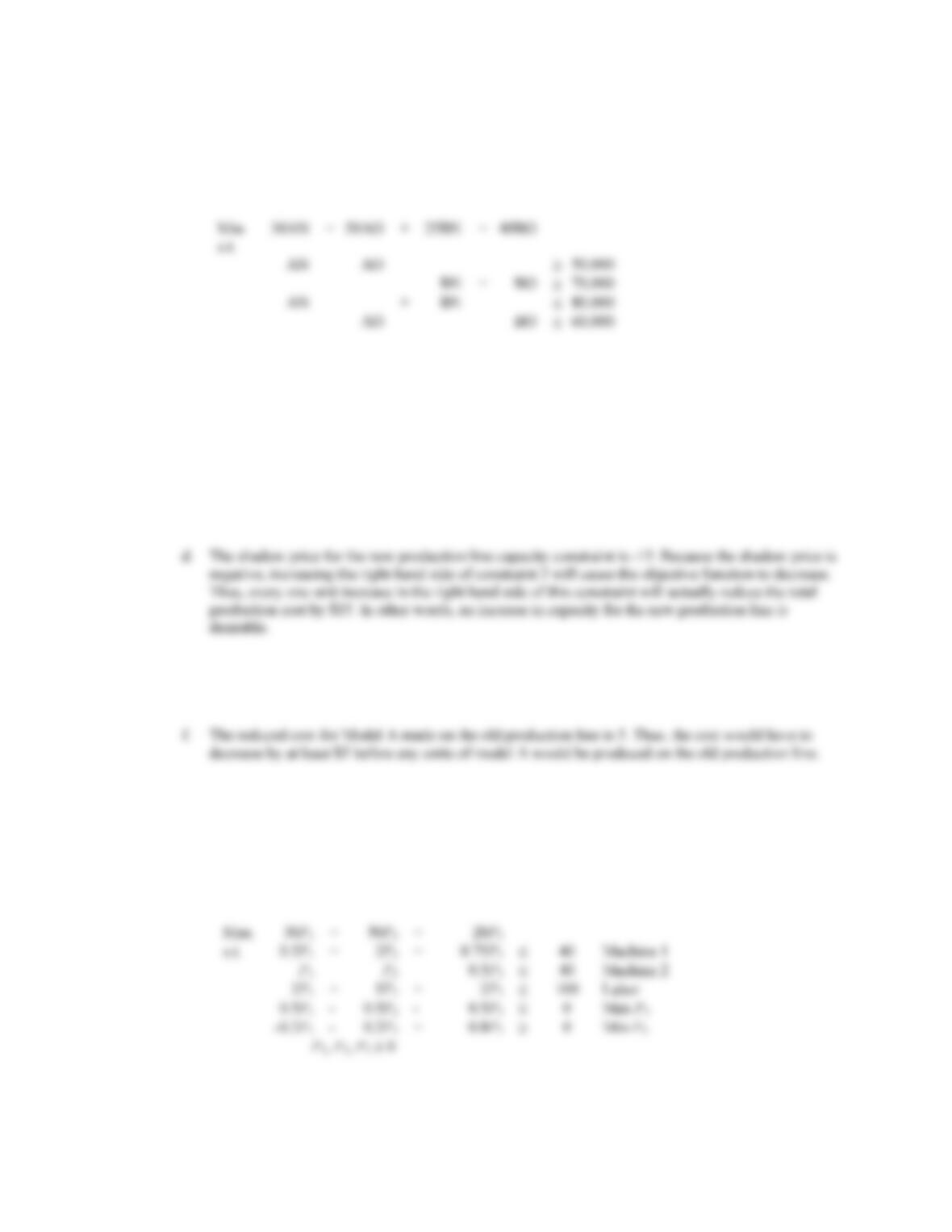
18. a. The linear programming model is as follows:
b. Optimal solution:
New Line
Old Line
Model A
50,000
0
Model B
30,000
40,000
Total Cost $3,850,000
c. The first three constraints are binding because the Final Values for these constraints are equal to the
R.H. Sides. The fourth constraint, with a slack of 20,000 is nonbinding.
e. Because constraint 4 is not a binding constraint, any increase in the production line capacity of the
old production line will have no effect on the optimal solution. Thus, there is no benefit in increasing
the capacity of the old production line.
g. The right hand side range for constraint 2 shows an allowable decrease of 40,000. Thus, if the
minimum production requirement is reduced 10,000 units to 60,000, the shadow price of 40 is
applicable. Thus, total cost would decrease by 10,000(40) = $400,000.
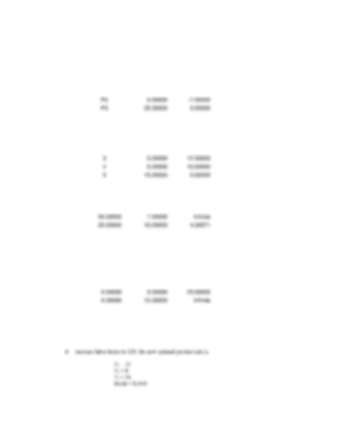
19. a. Let P1 = units of product 1
P2 = units of product 2
P3 = units of product 3
25BN
Markov Processes
8 – 9
The optimal solution is
Optimal Objective Value
1250.00000
Variable
Value
Reduced Cost
P1
25.00000
0.00000
P2
0.00000
P3
25.00000
0.00000
Constraint
Slack
Shadow Price
1
8.75000
0.00000
2
2.50000
0.00000
3
0.00000
12.50000
4
0.00000
10.00000
5
15.00000
0.00000
Objective
Allowable
Allowable
Coefficient
Increase
Decrease
30.00000
Infinite
10.00000
50.00000
7.50000
RHS
Allowable
Allowable
Value
Increase
Decrease
40.00000
Infinite
8.75000
40.00000
Infinite
2.50000
100.00000
6.66667
100.00000
0.00000
5.00000
25.00000
0.00000
15.00000
b. Machine Hours Schedule:
Machine 1 31.25 Hours
Machine 2 37.50 Hours
c. $12.50
Chapter 17
8 – 10
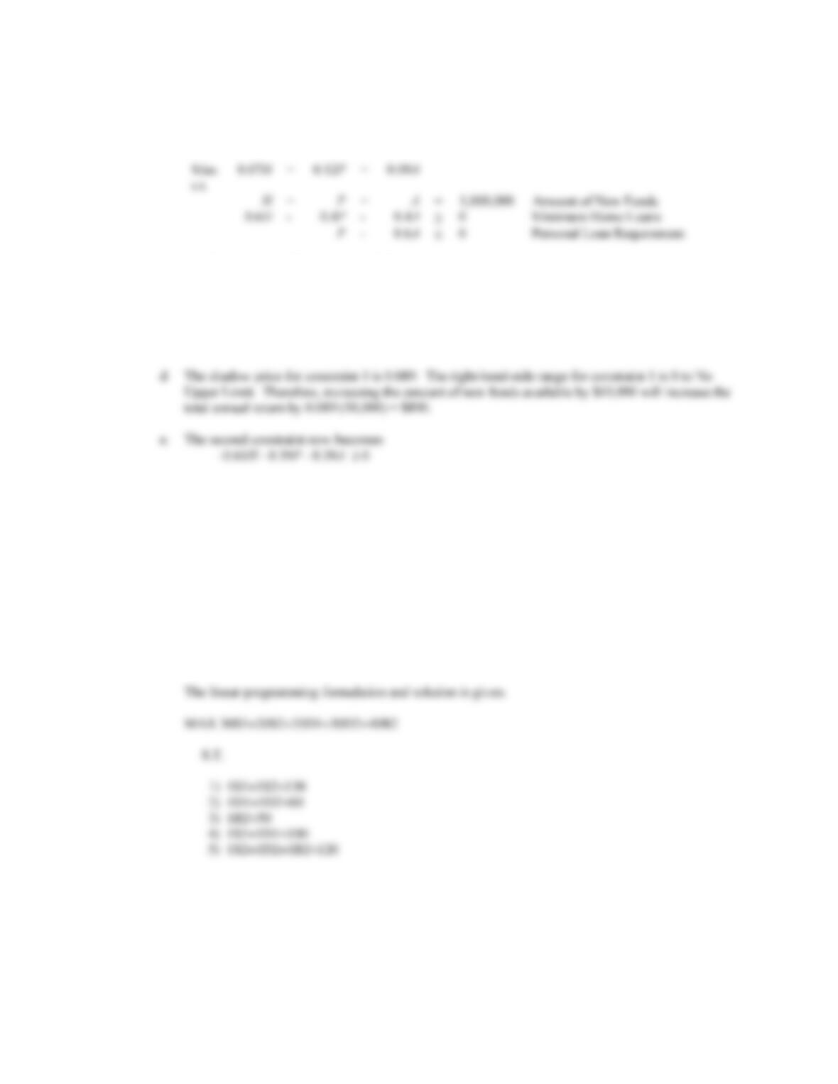
20. a. Let H = amount allocated to home loans
P = amount allocated to personal loans
A = amount allocated to automobile loans
b. H = $400,000 P = $225,000 A = $375,000
Total annual return = $88,750
Annual percentage return = 8.875%
c. The objective coefficient range for H is No Lower Limit to 0.101. Since 0.09 is within the range, the
solution obtained in part (b) will not change.
The new optimal solution is
H = $390,000 P = $228,750 A = $381,250
Total annual return = $89,062.50, an increase of $312.50
Annual percentage return = 8.906%, an increase of approximately 0.031%
21. a. Let S1 = SuperSaver rentals allocated to room type I
S2 = SuperSaver rentals allocated to room type II
D1 = Deluxe rentals allocated to room type I
D2 = Deluxe rentals allocated to room type II
B1 = Business rentals allocated to room type II