Markov Processes
8 – 11
The optimal solution is
Optimal Objective Value
7000.00000
Variable
Value
Reduced Cost
S1
100.00000
0.00000
D1
0.00000
-5.00000
S2
10.00000
0.00000
D2
60.00000
0.00000
50.00000
0.00000
Constraint
Slack
Shadow Price
1
20.00000
0.00000
2
0.00000
10.00000
3
0.00000
20.00000
4
0.00000
30.00000
5
0.00000
20.00000
Objective
Allowable
Allowable
Coefficient
Increase
Decrease
30.00000
Infinite
5.00000
35.00000
5.00000
Infinite
20.00000
5.00000
20.00000
30.00000
Infinite
5.00000
40.00000
Infinite
20.00000
RHS
Allowable
Allowable
Value
Increase
Decrease
130.00000
Infinite
20.00000
60.00000
10.00000
20.00000
50.00000
10.00000
20.00000
100.00000
20.00000
100.00000
120.00000
20.00000
10.00000
20 SuperSaver rentals will have to be turned away if demands materialize as forecast.
b. RoundTree should accept 110 SuperSaver reservations, 60 Deluxe reservations and 50 Business
reservations.
c. Yes, the effect of a person upgrading is an increase in demand for Deluxe accommodations from 60
to 61. From constraint 2, we see that such an increase in demand will increase profit by $10. The
added cost of the breakfast is only $5.
Chapter 17
8 – 12
e. Yes. We would need the forecast of demand for each rental class on the next night. Using the
demand forecasts, we would modify the right-hand sides of the first three constraints and resolve.
22. a. Let L = number of hours assigned to Lisa
D = number of hours assigned to David
S = amount allocated to Sarah
b. L = 48 hours D = 72 Hours S = 30 Hours
Total Cost = $3780
c. The shadow price for constraint 5 is 0. Therefore, additional hours for Lisa will not change the
solution.
23. a. Let C1 = units of component 1 manufactured
C2 = units of component 2 manufactured
C3 = units of component 3 manufactured
Max
+
+
The optimal solution is
C1 = 600
C2 = 700
C3 = 200
b.
Variable
Objective Coefficient Range
C1
No Lower Limit to 9.0
C2
C3
6.00 to No Lower Limit
5.33 to 9.0
Max
+
+
s.t.
+
+
=
Total Time
Markov Processes
8 – 13
Constraint
Right-Hand-Side Range
1
4400 to 7440
2
6300 to No Upper Limit
3
5
6
These are the ranges over which the shadow prices for the associated constraints are applicable.
d. Nothing, since there are 300 minutes of slack time on the grinder at the optimal solution.
e. No, since at that price it would not be profitable to produce any of component 3.
24. Let A = number of shares of stock A
a. To get data on a per share basis multiply price by rate of return or risk measure value.
Min
10A
+
3.5B
+
4C
+
3.2D
s.t.
100A
+
50B
+
80C
+
40D
=
200,000
Solution: A = 333.3, B = 0, C = 833.3, D = 2500
Risk: 14,666.7
Return: 18,000 (9%) from constraint 2
b.
Variable
Objective Coefficient Range
A
9.5 to 11
B
3.33 to No Upper Limit
C
D
3.2 to 4.4
No Lower Limit to 3.33
Individual changes in the risk measure coefficients within these ranges will not cause a change in the
optimal investment decisions.
Chapter 17
8 – 14
25. a. Let O1 = percentage of Oak cabinets assigned to cabinetmaker 1
O2 = percentage of Oak cabinets assigned to cabinetmaker 2
O3 = percentage of Oak cabinets assigned to cabinetmaker 3
C1 = percentage of Cherry cabinets assigned to cabinetmaker 1
C2 = percentage of Cherry cabinets assigned to cabinetmaker 2
C3 = percentage of Cherry cabinets assigned to cabinetmaker 3
Note: objective function coefficients are obtained by multiplying the hours required to complete all
the oak or cherry cabinets times the corresponding cost per hour. For example, 1800 for O1 is the
product of 50 and 36, 1764 for O2 is the product of 42 and 42 and so on.
b.
Cabinetmaker 1
Cabinetmaker 2
Cabinetmaker 3
Oak
O1 = 0.271
O2 = 0.000
O3 = 0.729
Cherry
C1 = 0.000
C2 = 0.625
C3 = 0.375
Total Cost = $3672.50
e. The new objective function coefficients for O2 and C2 are 42(38) = 1596 and 48(38) = 1824,
respectively. The optimal solution does not change but the total cost decreases to $3552.50.
26. a. Let M1 = units of component 1 manufactured
M2 = units of component 2 manufactured
+
+
+
+
+
+
+
+
+
Markov Processes
8 – 15
Min
4.50 M1
+
5.00M2
+
2.75M3
+
6.50P1
+
8.80P2
+
7.00P3
s.t.
2M1
+
3M2
+
4M3
21,600
Production
1M1
+
1.5M2
+
3M3
15,000
Assembly
+
+
Testing/Packaging
Component 1
+
Component 2
+
Component 3
b.
Source
Component 1
Component 2
Component 3
Manufacture
2000
4000
1400
Purchase
4000
0
2100
Total Cost: $73,550
d. The shadow price is $7.969. This tells us that the value of the optimal solution will increase by
$7.969 for an additional unit of component 2. Note that although component 2 has a purchase cost
per unit of $8.80, it would only cost Benson $7.969 to obtain an additional unit of component 2.
27. a. LP Formulation
The objective function maximizes the total revenue generated from wet-harvested cranberries and
dry-harvested cranberries. Each barrel of wet-harvested cranberries generates $17.50 in revenue;
dry-harvested cranberries earn $32.50 per barrel. The first constraint ensures that no more than
5,000 total barrels of cranberries are harvested. The second constraint states that every barrel of wet-
Max
17.5W+ 32.5D
W+D≤5,000 Total Harvest
.04W+.18D≤1,008 Dechaffing
.10W+.32D≤1,008 Cleaning
Chapter 17
The optimal solution is to harvest 2690.909 barrels of wet cranberries and 2309.091 barrels of dry
cranberries.
b. Below is the sensitivity analysis output for this problem:
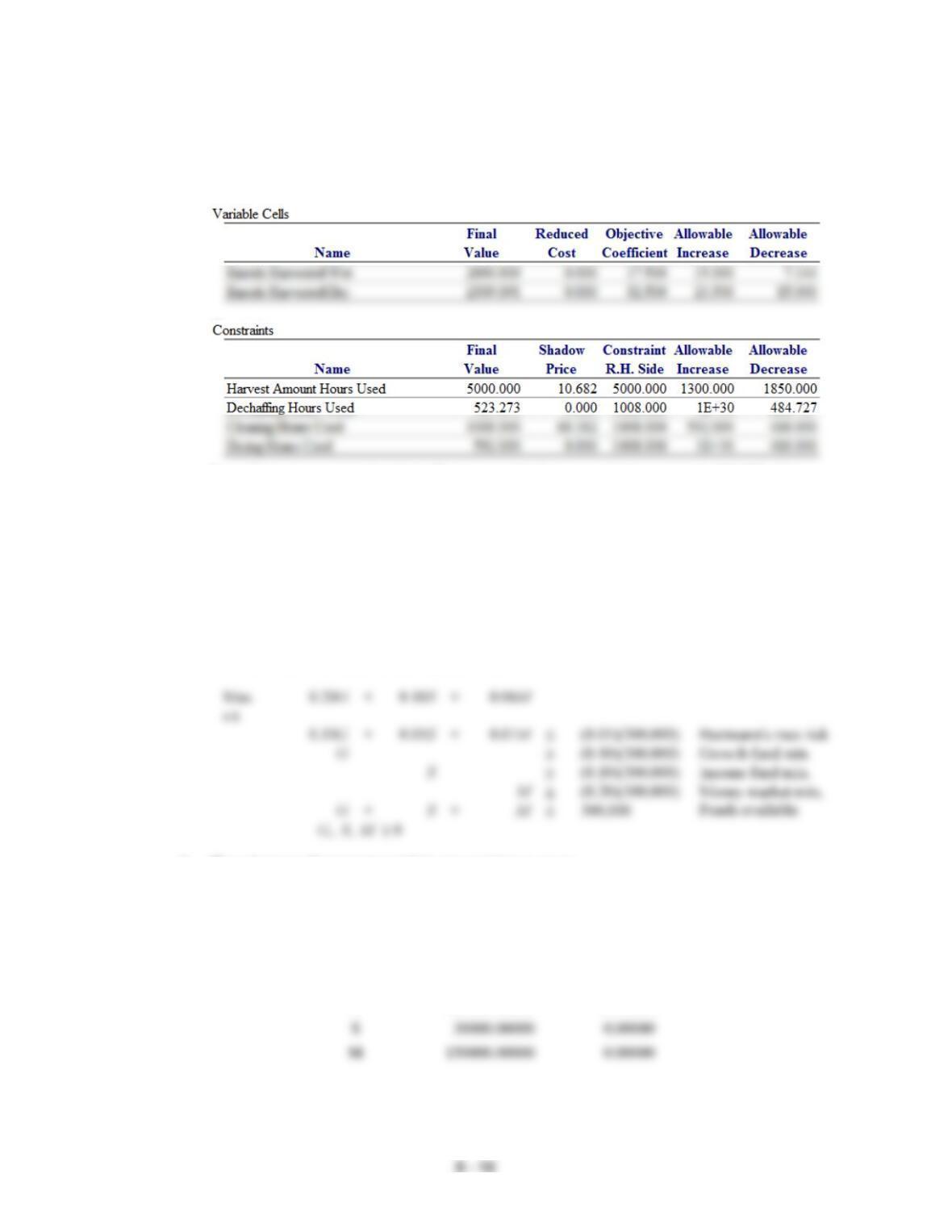
From this output, we see that dechaffing is not a binding constraint because only 523.273 of the
1008 available hours are being used. Fresh Made should not purchase additional dechaffing
capacity.
c. Assuming everything else remains unchanged, each additional hour of cleaning capacity added
(subtracted) from the 1,008 available hours increases (decreases) revenues $68.18. This is true for
any cleaning capacity value between 1008 – 416 = 592 and 1008 + 592 = 1600.
28. a. Let G = amount invested in growth stock fund
S = amount invested in income stock fund
M = amount invested in money market fund
b. The solution to Hartmann’s portfolio mix problem is given.
Optimal Objective Value
36000.00000
Variable
Value
Reduced Cost
G
120000.00000
0.00000
30000.00000
0.00000
M
150000.00000
0.00000
Markov Processes
8 – 17
Constraint
Slack
Shadow Price
1
0.00000
1.55556
2
90000.00000
0.00000
3
0.00000
4
90000.00000
0.00000
5
0.00000
0.12000
Objective
Allowable
Allowable
Coefficient
Increase
Decrease
0.20000
Infinite
0.05000
0.10000
0.02222
1.20000
0.06000
0.14000
0.04000
RHS
Allowable
Allowable
Value
Increase
Decrease
0.00000
8100.00000
8100.00000
0.00000
90000.00000
Infinite
0.00000
162000.00000
30000.00000
0.00000
90000.00000
Infinite
300000.00000
Infinite
300000.00000
c. These are given by the objective coefficient ranges. The portfolio above will be optimal as long as
the yields remain in the following intervals:
Growth stock 0.15 c1 0.60
Income stock No Lower Limit < c2 0.122
Money Market 0.02 c3 0.20
e. This change is outside the objective coefficient range so we must re-solve the problem. The solution
is shown below.
Chapter 17
8 – 18
LINEAR PROGRAMMING PROBLEM
MAX .1G + .1S + .06M
S.T.
1) .1G + .05S + .01M < 15000
2) G > 30000
OPTIMAL SOLUTION
Optimal Objective Value
27600.00000
Variable
Value
Reduced Cost
G
30000.00000
0.00000
S
210000.00000
0.00000
M
60000.00000
0.00000
Constraint
Slack
Shadow Price
1
900.00000
0.00000
2
0.00000
0.00000
3
180000.00000
0.00000
4
0.00000
5
0.00000
0.09200
Objective
Allowable
Allowable
Coefficient
Increase
Decrease
0.10000
0.00000
0.92000
0.10000
Infinite
0.00000
0.06000
0.04000
0.33498
RHS
Allowable
Allowable
Value
Increase
Decrease
0.00000
Infinite
900.00000
0.00000
18000.00000
30000.00000
0.00000
180000.00000
Infinite
0.00000
180000.00000
22500.00000
300000.00000
Infinite
299999.99999
Markov Processes
8 – 19
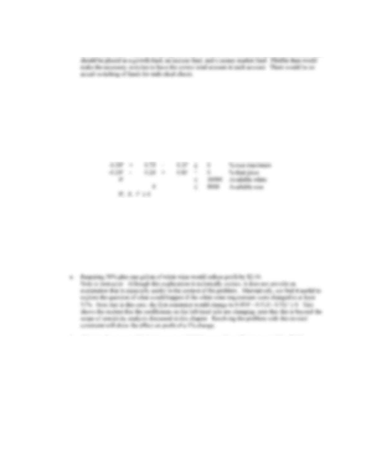
g. With the new yield estimates, Pfeiffer would solve a new linear program to find the optimal portfolio
mix for each client. Then by summing across all 50 clients he would determine the total amount that
29. a. Relevant cost since LaJolla Beverage Products can purchase wine and fruit juice on an as – needed
basis.
b. Let W = gallons of white wine
R = gallons of rose wine
F = gallons of fruit juice
Max
1.5 W
+
1R
+
2F
s.t.
0.5W
–
0.5R
–
0.5F
0
% white
-0.3W
+
0.7R
–
0.3F
0
–
+
=
0
10000
Available white
8000
Available rose
-0.2W
+
0.8R
–
0.2F
0
% rose minimum
Optimal Solution: W = 10,000, R = 6000, F = 4000
profit contribution = $29,000.
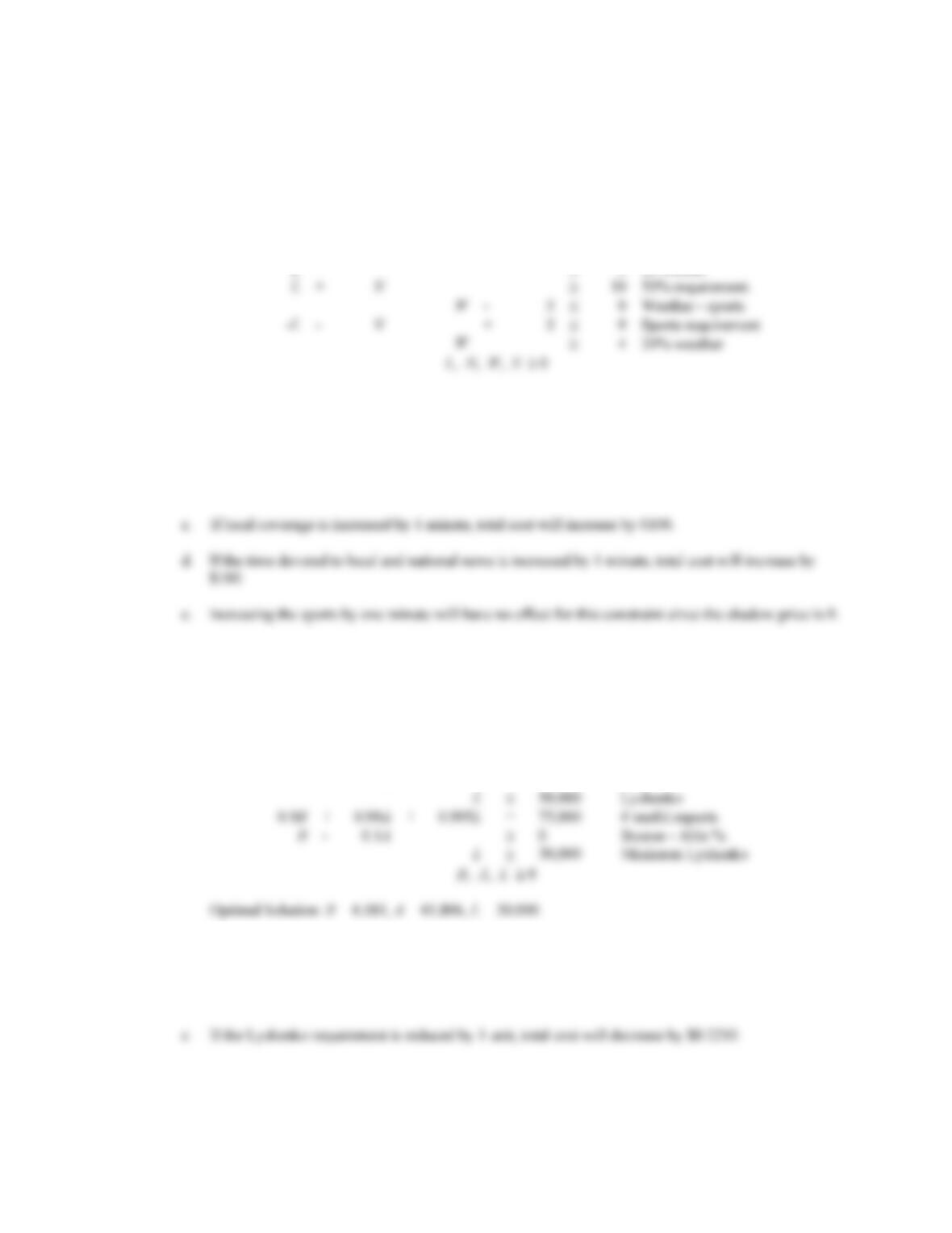
c. Since the cost of the wine is a relevant cost, the shadow price of $2.90 is the maximum premium
(over the normal price of $1.00) that LaJolla Beverage Products should be willing to pay to obtain
one additional gallon of white wine. In other words, at a price of $3.90 = $2.90 + $1.00, the
additional cost is exactly equal to the additional revenue.
d. No; only 6000 gallons of the rose are currently being used.
f. Allowing the amount of fruit juice to exceed 20% by one gallon will increase profit by $1.00.
Chapter 17
8 – 20
30. a. Let L = minutes devoted to local news
N = minutes devoted to national news
W = minutes devoted to weather
S = minutes devoted to sports
Min
300L
+
200N
+
100W
+
100S
s.t.
L
+
N
+
W
+
S
=
20
Time available
15% local
–
Weather – sports
–
Sports requirement
20% weather
Optimal Solution: L = 3, N = 7, W = 5, S = 5
Total cost = $3,300
b. Each additional minute of broadcast time increases cost by $100; conversely, each minute reduced
will decrease cost by $100. These interpretations are valid for increase up to 10 minutes and
decreases up to 2 minutes from the current level of 20 minutes.
31. a. Let B = number of reservoir capacitors awarded to Boston Components
A = number of reservoir capacitors awarded to Able Controls
L = number of reservoir capacitors awarded to Lyshenko Industries
Min
2.45B
+
2.5A
+
2.75L
s.t.
B
30,000
Boston
A
50,000
Able
50,000
Lyshenko
0.9B
+
0.99A
+
0.995L
75,000
# useful reports
B
–
0
Boston – Able %
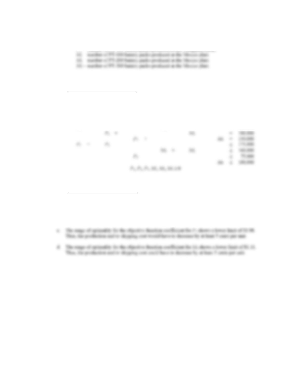
b. Suppose that Boston Components has a defective rate of 2% instead of 10%. The new optimal
solution would increase the volume assigned to Boston Components to 30,000 capacitors. In this
case, the additional units assigned to Boston Components would reduce on a one-for-one basis the
number assigned to Able Controls.
Markov Processes
8 – 21
32. a. Let P1 = number of PT-100 battery packs produced at the Philippines plant
P2 = number of PT-200 battery packs produced at the Philippines plant
Total production and shipping costs ($/unit)
Philippines
Mexico
PT-100
1.13
1.08
PT-200
1.16
1.16
PT-300
1.52
1.25
Min
1.13P1
+
1.16P2
+
1.52P3
+
1.08M1
+
1.16M2
+
1.25M3
s.t.
P1
+
M1
=
200,000
+
=
100,000
+
M3
=
150,000
b. The optimal solution is as follows:
Philippines
Mexico
PT-100
40,000
160,000
PT-200
100,000
0
PT-300
50,000
100,000
The total production and transportation cost is $535,000.
Chapter 17
8 – 22