9. The Excel workbook C08 Problem Data provides data on quality losses at Nosoco Paper
Mill. Find the percentage of cost for each category, and the cumulative percentages when
the categories are sorted by decreasing costs. Construct an appropriate Excel chart to
analyze the data. What conclusions do you reach?
See Excel file Problem 8.9 in the instructor materials.
Sorted by cost:
Category
Cost
Percent
Cumulative %
Rejected paper
$375,000
57.25%
57.25%
Customer complaints
$103,000
15.73%
72.98%
Odd lot
$66,000
10.08%
83.05%
$31,000
87.79%
Downtime
$30,000
92.37%
Inspection
$25,000
96.18%
Quality improvement training
$10,000
$655,000
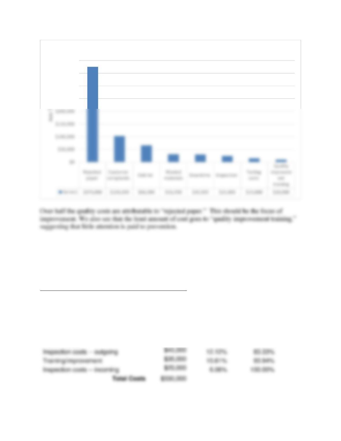
10. Stateside Metrology Repairs, Inc. has a thriving business repairing and upgrading high–
technology measuring instruments. The costs of quality that they have collected over the
past year can be found in the Excel workbook C08 Problem Data. Analyze their quality
losses and to suggest which areas they should address first in an effort to improve their
quality.
See Excel file Problem 8.10 in the instructor materials.
Cost
Percent
Cumulative %
Customer returns
$120,000
36.36%
36.36%
Workstation downtime
$60,000
18.18%
54.55%
Rework costs
$55,000
16.67%
71.21%
Inspection costs — outgoing
$40,000
12.12%
83.33%
Training/improvement
$35,000
10.61%
93.94%
Inspection costs — incoming
$20,000
$330,000
$250,000
$300,000
$350,000
$400,000
Quality Cost Categories
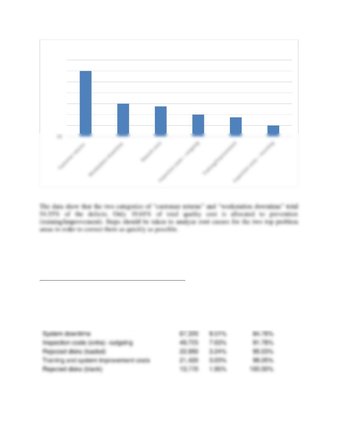
11. Analyze the quality losses at Beechware Software Corp. using the data in the Excel
workbook C08 Problem Data. What conclusions do you reach?
See Excel file Problem 8.11 in the instructor materials.
Category
Annual Loss
Percent
Cumulative %
Customer returns
$275,400
38.92%
38.92%
Rework
153,000
21.62%
60.54%
Inspection costs (extra)—incoming
104,040
14.70%
75.24%
System downtime
84.76%
Inspection costs (extra)—outgoing
91.78%
Rejected disks (loaded)
95.03%
Training and system improvement costs
98.05%
Rejected disks (blank)
$20,000
$40,000
$60,000
$80,000
$100,000
$120,000
$140,000
Quality Costs
12. A genetic researcher at GenLab, Ltd. is trying to test two laboratory thermometers
(that can be read to 1/100,000th of a degree Celsius) for accuracy and precision. She
measured 25 samples with each and obtained the results found in the C08 Problem Data
workbook. The true temperature being measured is 0º C. Compute the average and
variance of the data for each thermometer. Which instrument is more accurate? Which is
more precise? Which is the better instrument?
See Excel file Problem 8.12 in the instructor materials.
Thermometer A:
Average
0.00031
Variance
1.80251E-06
Average
Variance
1.45153E-06
Thermometer B is more accurate. In addition, the variance is smaller indicating that it is also
more precise. This can also be seen from the histograms of the data:
$0
$50,000
$100,000
$150,000
$200,000
$250,000
$300,000
Quality Costs
13. Two scales were at Aussieburgers, Ltd. used to weigh the same 25 samples of
hamburger patties for a fast-food restaurant in Australia. Results are shown in the C08
See Excel file Problem 8.13 in the instructor materials.
Scale A:
Average
116.32
4
6
8
Thermometer A
Frequency
4
6
8
10
Frequency
Thermometer B
Frequency
Scale B:
Average
113.96
6
8
10
12
Scale A
Frequency
4
5
6
7
8
9
Scale B
Frequency
Variance
Relative error
14. A gauge repeatability and reproducibility study at NewGauge, Inc., collected data for
three operators, two trials, and eight parts, available in the C08 Problem Data worksheet.
The part specification is 1.5 ± 0.1 inches. Use formulas (8.6) through (8.24) to analyze these
data, and check your answers using the R&R Excel template (some differences will exist
due to rounding). Interpret the results.
See Excel file Problem 8.14 in the instructor materials.
The Excel template results are shown in the Excel file noted above. This exercise is focused on
helping students to understand the formulas and their implementation. Manual calculations are
shown below.
x
1 = (Mijk) /nr = 23.940 /16 = 1.496
R
1 = (Rij) / n = 0.148 /8 = 0.019
x
2 = 24.008 / 16 = 1.501;
R
2 = 0.246/8 = 0.031
Finally, to calculate values for the third operator:
EV = K1
R
= (4.56) (0.028) = 0.126
AV =
(K x ) – (EV / nr)
2D
2 2
=
/16)([0.126] – [0.013]) ([2.70] 22
= 0.015
% of Total Variation:
Equipment variation = 100 0.126
0.136 = 92.65%
x
R
R
Part variation = 100 0.048
0.136 = 35.29%
% of Tolerence
Equipment variation = 100 0.126
0.20 = 63.00%
Variance Ratios
EV% of Total Variance = 100 𝐸𝑉2
𝑇𝑉2 = 100 0.1262
01362 = 85.8%
15. A gauge repeatability and reproducibility study at Frankford Brake Systems collected
the data available in the C08 Problem Data workbook. The part specification is 1.0 ± 0.06
mm. Analyze these data using the R&R Excel template and interpret the results.
See Excel file Problem 8.15 in the instructor materials.
Although students will use the Excel template (results are shown in the Excel file noted above),
instructors might wish to discuss the formulas or have students verify the results using them
similar to Problem 8.14. The manual calculations are shown below. Some differences exist due
to rounding.
x
1 = (Mijk) /nr = 29.720 / 30 = 0.9907;
R
1 = (Rij) / n = 0.280 / 10 = 0.028
x
R
x
x
x
D4 = 2.574; UCLR = D4
R
= (2.574) (0.033) = 0.0849, all ranges below
K1 = 3.05 ; K2 = 3.65 (from Table 8.3)
EV = K1
R
= (3.05) (0.033) = 0.101
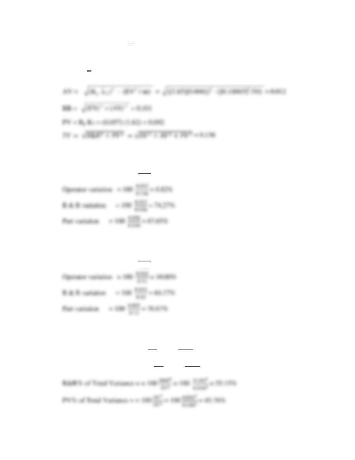
% of TV
Equipment variation = 100 0.101
0.136 = 74.27%
% of Tolerance
Equipment variation = 100 0.101
0.12 = 84.17%
Variance Ratios
EV% of Total Variance = 100 𝐸𝑉2
𝑇𝑉2 = 100 0.1012
01362 = 55.15%
AV% of Total Variance = = 100 𝐴𝑉2
𝑇𝑉2 = 100 0.0122
0.1362 = 0.78%
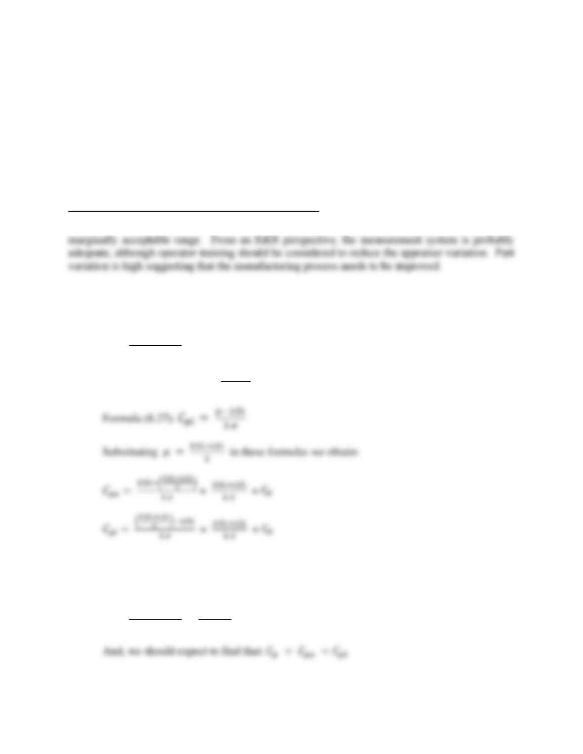
Equipment variation is unacceptable; operator variation is OK. The company should focus on
the repeatability issue.
16. A gauge repeatability and reproducibility study was made at Accurate Parts, Inc., using
three operators, taking three trials each on identical parts. The data can be found in the
C08 Problem Data workbook. The part specification for the collar that was measured was
1.6 ± 0.2 inches. Analyze these data using the R&R Excel template and interpret the
results.
See Excel file Problem 8.16 in the instructor materials.
From the results, repeatability (EV) is acceptable; and reproducibility (AV) falls in the
17. Use formulas (8.26) and (8.27) to show mathematically that when the process mean is
centered between LSL and USL, Cpu = Cpl = Cp.
𝜇 = 𝑈𝑆𝐿+𝐿𝑆𝐿
2
Formula (8.26): 𝐶𝑝𝑢 = 𝑈𝑆𝐿−µ
3 𝜎
This can be shown most easily by taking a numeric example. If LSL = 4 and USL = 10 and the
estimated value of = 1, then µ =7, if the process mean is centered.
𝜇 = 𝑈𝑆𝐿+𝐿𝑆𝐿
2= 10+4
2=7
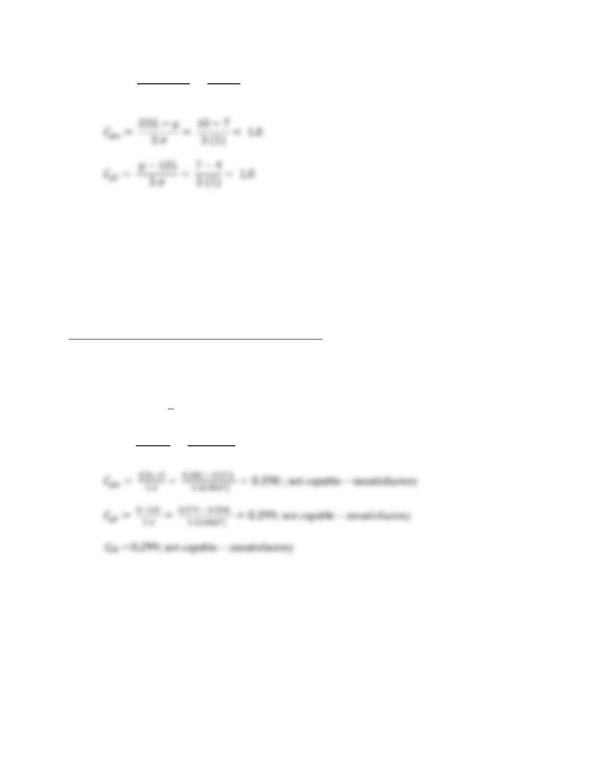
𝐶𝑝 = 𝑈𝑆𝐿−𝐿𝑆𝐿
6 𝜎 = 10−4
6 (1) =1.0
18. A machining process at the Mach4 Tool Co. has a required dimension on a part of 0.575
± 0.007 inch. Dimensions of twenty-five parts were measured and are available in the C08
Problem Data workbook.
a. Compute the process capability indexes using formulas (8.25) through (8.28) and
interpret the results.
b. Adjustments were made in the process and 25 more samples were taken and measured,
which are also provided in the data file. What can you observe about the process? Is it now
capable of producing within acceptable limits?
See Excel file Problem 8.18 in the instructor materials.
Students may use the Process Capability Excel template, but should also be able to do the
calculations by hand (differences due to rounding).
a. Sample statistics:
x
= 0.5740; = 0.0067 and a tolerance of 0.575 ± 0.007.
𝐶𝑝 = 𝑈𝑆𝐿−𝐿𝑆𝐿
6 𝜎 = 0.582−0.568
6 (0.0067)=0.3483 ; not capable – unsatisfactory
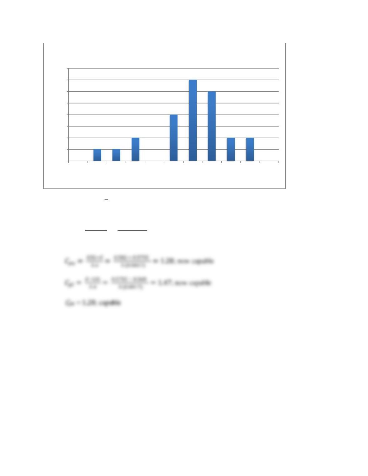
b. Sample statistics:
x
= 0.5755; = 0.0017 and the same tolerance of 0.575 ± 0.007 and shows
that the standard deviation is smaller than previously, indicating less variation within the data.
𝐶𝑝 = 𝑈𝑆𝐿−𝐿𝑆𝐿
6 𝜎 = 0.582−0.568
6 (0.0017)=1.373; the process capability is now satisfactory
0
1
2
3
4
5
6
7
8
0.5550 0.5585 0.5620 0.5655 0.5690 0.5725 0.5760 0.5795 0.5830 0.5865 0.5900
Frequency
Cell Upper Limit
Histogram
19. From the data for Saramit Theatrical Products that can be found in the C08 Problem
Data workbook, use the Process Capability Excel template to find a histogram and compute
the process capability indexes. If the specifications are 22 ± 0.03, estimate the percentage of
parts that will be nonconforming assuming a normal distribution.
See Excel file Problem 8.19 in the instructor materials.
Process Capability Index Calculations
Average
22.0012
Standard deviation
0.0089
Cp
1.1281
Cpl
1.1749
Cpu
1.0812
Cpk
1.0812
3
4
5
6
7
Histogram
For sample statistics:
x
= 22.0012; σ= 0.0089
Specification limits are 21.97 and 22.03
Use NORM.DIST (22.0300, 22.0012, 0.0089, TRUE) to find the P(z < 3.24) = 0.9994
𝑧=𝐿𝑆𝐿−𝑥̅
𝜎= 21.9700−22.0012
0.0089 =−3.51
20. Samples for three parts made at River City Parts Co. were taken and provided in the
C08 Problem Data workbook.
See Excel file Problem 8.20 in the instructor materials.
20
25
30
Histogram
a. Calculate the mean and standard deviation for each part and compare the natural
variation of each part to the following specification limits:
Part Nominal Tolerance
1 1.750 ± 0.045
2 2.000 ± 0.060
3 1.250 ± 0.030
Sample statistics as shown in spreadsheet Prob.08-20.xlsx in the Instructor materials are:
Part 1:
x
= 1.7446; s = 0.0163; 3s = 0.0489
b. Will the production process permit an acceptable fit of all parts into a slot with a
specification of 5 ± 0.081 at least 99.73 percent of the time?
x
T = 𝑥̅1+𝑥̅2 + 𝑥̅3 = 4.9930
Estimated Process =
sss 2
3
2
2
2
1++
=
0.0163 +0.0078 +0.0052
2 2 2
= 0.0188
21. Suppose that a refrigeration process at Coldfoods, Ltd., has a normally distributed
output with a mean of 27.0 and a variance of 1.21.
a. If the specifications are 27.0 ± 3.25, compute Cp, Cpk, and Cpm. Is the process capable and
centered?
x
= 27.0; = 1.1
x
𝐶𝑝𝑢 = 𝑈𝑆𝐿−𝑥̅
3 𝜎 = 30.25 − 27.00
3 (1.1) =0.985
b. Suppose the mean shifts to 26.0 but the variance remains unchanged. Recompute and
interpret these process capability indexes.
x
= 26; = 1.1
𝐶𝑝= 𝑈𝑆𝐿−𝐿𝑆𝐿
6 𝜎 = 30.25 − 23.75
6 (1.1) =0.985
𝐶𝑝𝑚 = 𝐶𝑝
√1+[(𝑚𝑒𝑎𝑛−𝑡𝑎𝑟𝑔𝑒𝑡)2
𝜎2]= 0.985
√1+[(26.0−27.0)2
(1.1)2]=0.729
Because of the shift away from the target, capability is lower.
𝐶𝑝𝑢 = 𝑈𝑆𝐿−𝑥̅
3 𝜎 = 30.25 − 26.00
3 (1.1) =1.288
c. If the variance can be reduced to 40 percent of its original value, how do the process
capability indices change (using the original mean of 27.0).
2
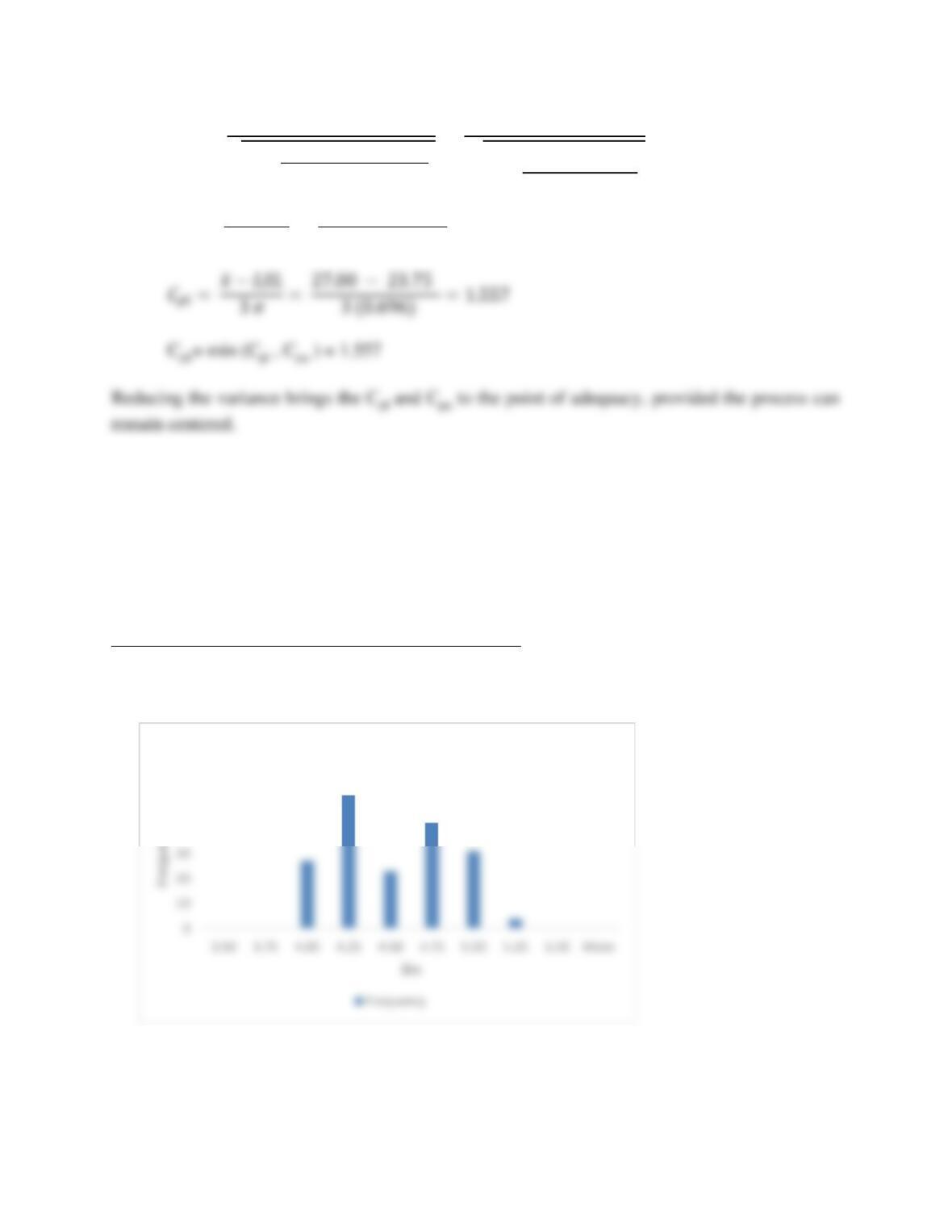
𝐶𝑝𝑚 = 𝐶𝑝
√1+[(𝑚𝑒𝑎𝑛−𝑡𝑎𝑟𝑔𝑒𝑡)2
𝜎2]= 1.557
√1+[(27.0−27.0)2
(0.696)2]=1.557
𝐶𝑝𝑢 = 𝑈𝑆𝐿−𝑥̅
3 𝜎 = 30.25 − 27.00
3 (0.696)=1.557
22. River Bottom Fire Department is evaluating their response times in order to determine
whether a new fire station is needed. Samples were taken for 30 consecutive days from 6
stations. These data can be found in the C08 Problem Data workbook.
a. Compute the mean and standard deviation, and construct a histogram for these 180
individual readings.
b. Construct a run chart for the sample means.
c. Interpret the results.
See Excel file Problem 8.22 in the instructor materials.
a) The mean is 4.40 and the standard deviation is 0.351. The histogram is shown below.
b)
40
50
60
Histogram
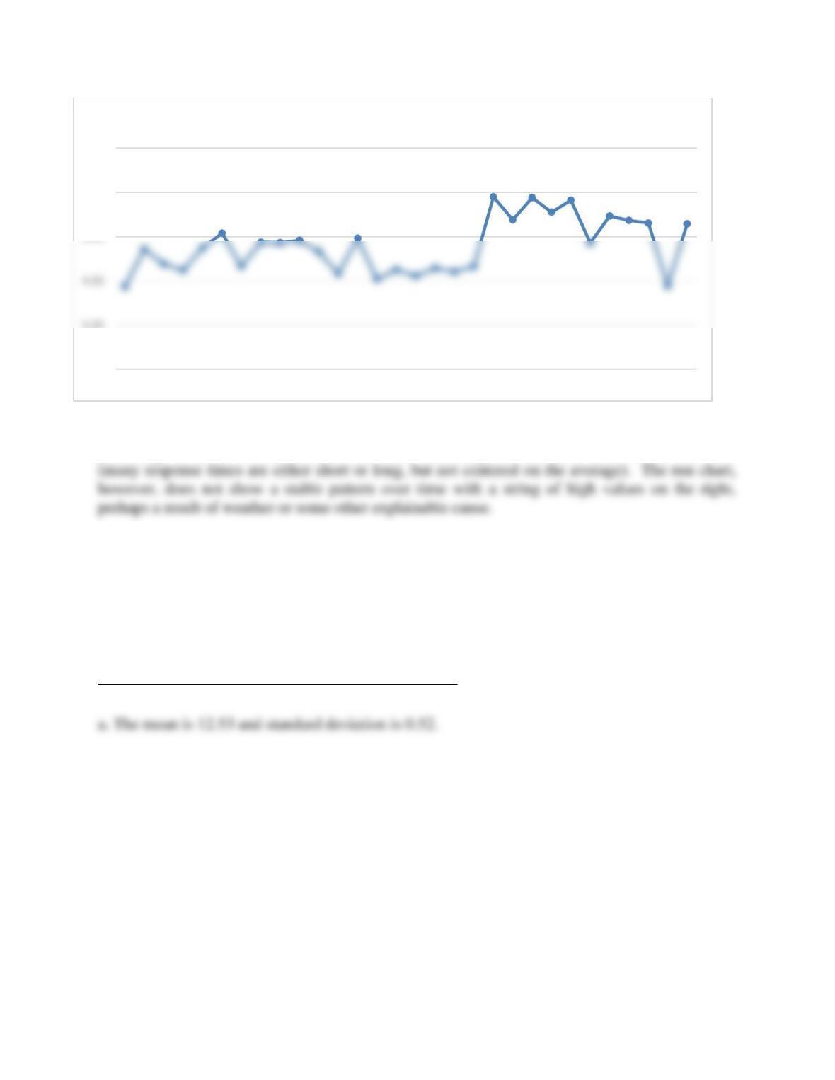
c) The histogram suggests a somewhat symmetric, but not bell-shaped, distribution with a larger
percentage of values above and below the mean. This might be a result of the stations’ locations
23. Palma State Bank is investigating the processing time for loan applications. Samples
were taken for 25 random days from 5 branches. These data can be found in the C08
Problem Data workbook.
a. Compute the mean and standard deviation, and construct a histogram for these data.
b. Construct a run chart for the sample means
c. Interpret the results.
See Excel file Problem 8.23 in the instructor materials.
3.00
3.50
5.00
5.50
12345678910 11 12 13 14 15 16 17 18 19 20 21 22 23 24 25 26 27 28 29 30
Run Chart
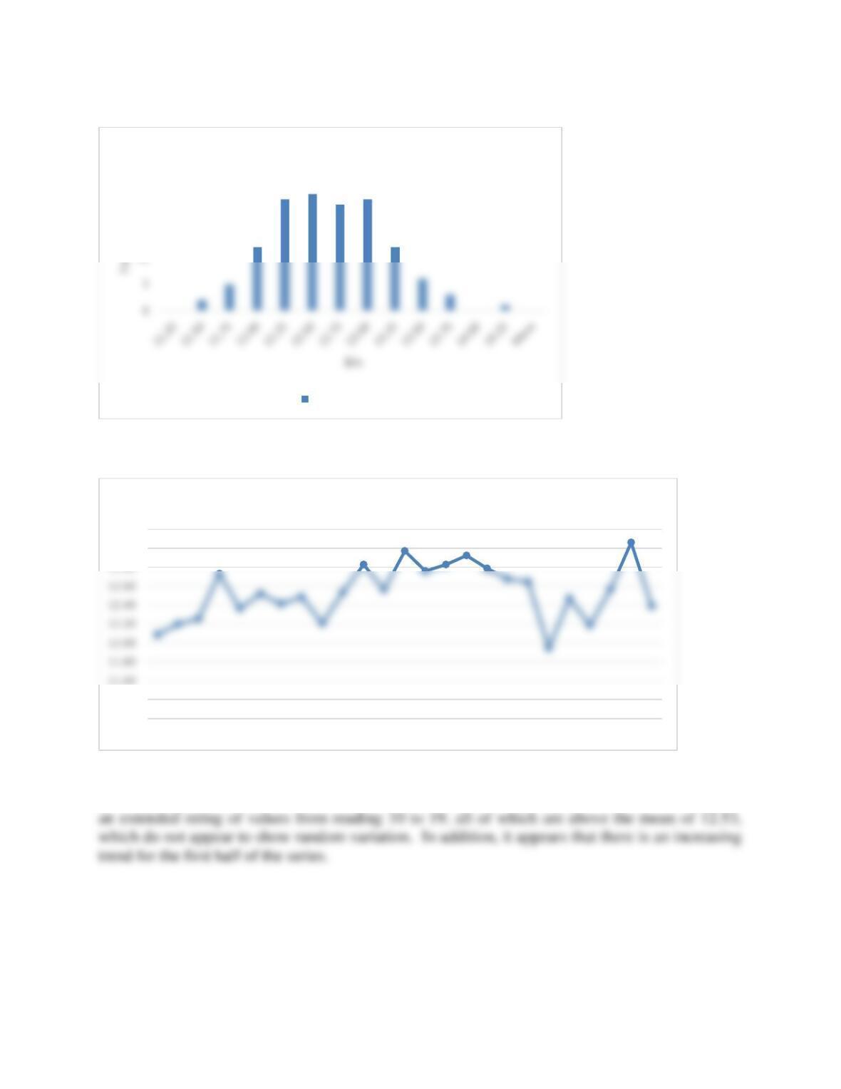
b) The run chart of sample means is shown below.
c) The histogram shows that the data is fairly symmetric and bell-shaped around the mean. It has
24. Birdseye Magnetronics makes induction meters used in vending machines to test the
validity of coins. Their specifications require the induction reading capability of the meters
to fall between 0.25 and 0.50 Tesla (T) units. Quality analysts took 3 random test readings
of 30 meters, available C08 Problem Data workbook.
a. Compute the mean and standard deviation, and construct a histogram for these data.
10
15
20
25
Histogram
Frequency
11.20
11.40
13.00
13.20
1 2 3 4 5 6 7 8 9 10 11 12 13 14 15 16 17 18 19 20 21 22 23 24 25
Run Chart
b. Construct a run chart for the sample means
c. Interpret the results.
See Excel file Problem 8.24 in the instructor materials.
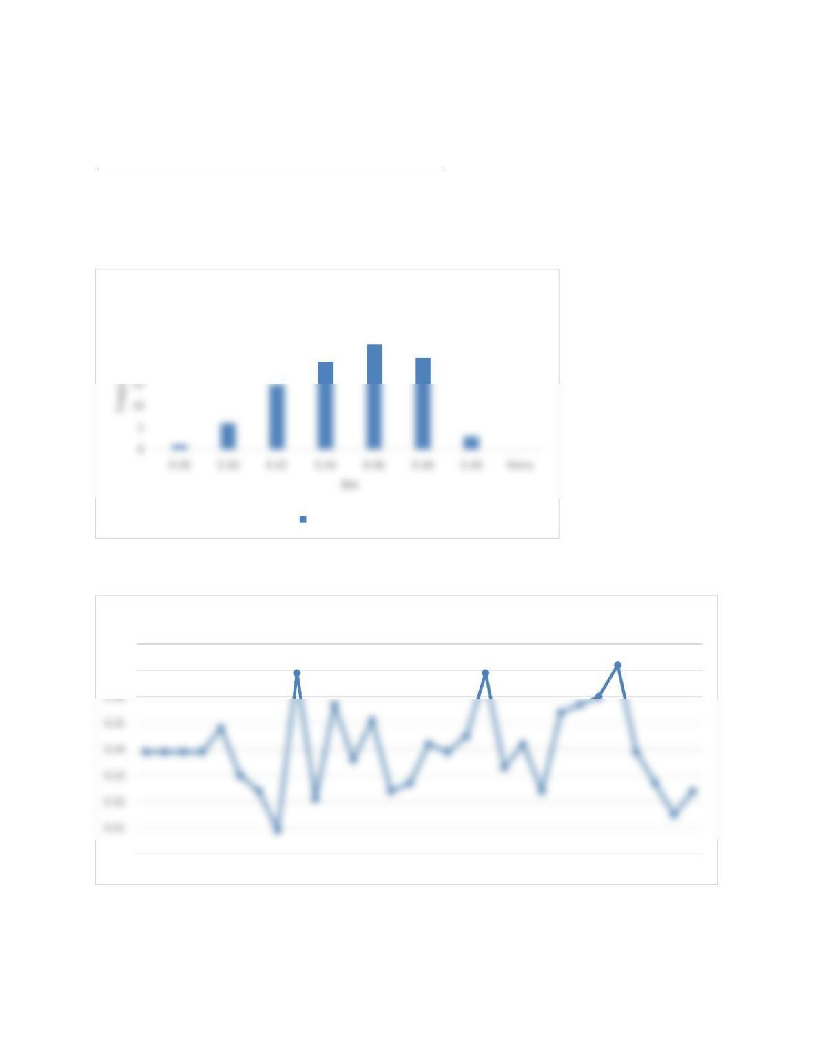
a. The mean for all the values is 0.340, and all data lie within the specifications. However, the
histogram show some negative (left) skewness.
b.
20
25
30
Histogram
Frequency
0.30
0.37
0.38
12345678910 11 12 13 14 15 16 17 18 19 20 21 22 23 24 25 26 27 28 29 30
Run Chart