MBPF Ch7 solutions. Last updated: August 28, 2011
61
CHAPTER 7: MANAGING FLOW VARIABILITY: SAFETY
INVENTORY
7.1 Objective
In the previous chapter on inventory, we focused on economies of scale as the major driver for
inventory. The purpose of this chapter is to introduce the notion of safety inventory as a buffer
against stochastic variability in supply / demand and discuss various levers for reducing it.
The chapter is covered over two classes each of duration 100 minutes. In the first class, we first
motivate the need for forecasting as a way of estimating demand. We emphasize the four key
Thus the supply chain module occupies three 100 minutes classes, one based on chapter 6 and
two based on chapter 7.
7.2 Additional Suggested Readings
We continue with the Hewlett-Packard case to illustrate the notion of safety stock and the
concept of centralization (across DCs in Europe).
Suggested assignment questions (continued from chapter 6):
1. Are there any other factors that need to be considered when deciding on the inventory
• Benetton (A), Harvard Business School case # 9-685-014.
Suggested questions:
1. Summarize the important elements of Benetton’s marketing, logistics, manufacturing and
This case can be used to all of the concepts in Chapters 6 and 7 including EOQ, centralization, as
well as the newsvendor model. The questions are part of the case.
7.3 Solutions to the Problem Set
Problem 7.1
[a] Given quantities: mean weekly demand = 400; standard deviation of weekly demand =
[b] The standard deviation of lead time demand,
LTD = 125 units. For each service level the
z-value can be read from the standard normal table. The safety inventory
Isafety = z x
LTD Finally, ROP = 400 + Isafety.
Problem 7.2
[a] Average weekly demand (R) = 1000
Standard deviation of weekly demand (
R) = 150.
Lead time (L) = 4 weeks.
[b] We use the EOQ formula to determine the optimal order quantity.
H = $1 * 25%/year = $.25/year
[c] If lead time (L) reduces to 1 week, then standard deviation of demand during lead time
Problem 7.3
(a) The optimal order quantity of planters for HG is
(c) Quantify the impact of the change.
Additional transportation cost per year = 1500*52*.2 = $15,600
Problem 7.4
First, is this an EOQ problem? Well, notice that the question dictates that we do a run
every two years. That would mean, in a deterministic EOQ setting, that Q must equal two
years of mean demand, i.e., 32000. Hence, this question does not give us the freedom to
change when we do a run (which is what EOQ is all about).
Thus, the question is whether 32000 is the best quantity we can print every two years?
This thus asks about what the appropriate safety stock (or service level) should be. We
know that this is answered by newsvendor logic. Answer these two questions:
1. What is my underage cost (cost of not having enough)? I.e., if I were to stock one
The last step is to convert the SL into a printing quantity. Recall that total average
demand for 2 years (R) = 32,000 with a standard deviation of 5656.86. The optimal
printing quantity, Q* is determined such that
Problem 7.5
The revenue per crate, p = $120.00, variable cost, c = $18.00, and salvage value, v = – $2.00. The
marginal benefit of stocking an additional crate (MB) = p – c = $120 – $18 = $102. The marginal
MB/(MB+MC) = 102/(102+20) = 0.836.
The probability density of demand and its cumulative probability is listed below.
Demand
0
1
2
3
4
5
6
7
8
9
10
11
12
13
14
15
The optimal order quantity is the smallest number of crates such that cumulative probability is at
least 0.836. From the table this gives the number of crates to be 12.
Problem 7.6
How many crews should the city assign to trash collection? For simplicity, you may treat the
number of crews as a continuous variable. For example, 4.1 crews would be a perfectly acceptable
answer.
One solution approach (starting from the basics):
Note that the marginal cost of scheduling one more ton = $125/ton.
Another approach to get the critical fractile probability SL uses the newsvendor solution directly:
Here we are stocking up on local trash collection capacity.
Problem 7.7 (This is an advanced problem)
We are concerned about the overbooking problem; that is, how many seats to overbook. The
randomness in demand arises from uncertain cancellations, which are uniformly distributed
between 0 and 20. One can think of this question as asking “what is the optimal service level of
cancellations?”
Prob.
0
0
0
Prob.
0
0
0
1
• If there are fewer cancellations than “stocked,” there are insufficient seats for those passengers
Problem 7.8
[a] To compute the optimal order quantity at each store we use the EOQ formula.
Assume 50 sales weeks/year.
[b] To compute the optimal order quantity at centralized store observe that this store
faces a cumulative average weekly demand = 4 x 10,000 = 40,000. This gives an annual
demand of 2,000,000 units.
Problem 7.9
(a) Given that each outlet orders independently and gets its own delivery, the optimal order size
at each outlet is
(b) On average, each unit spends
T = I / R = (Q/2) / R = 1,500 / 4000 weeks = 3/8 weeks = .375 weeks in the Hi-Tek system
before being sold
Problem 7.10
Mean demand, 1000/day with a daily standard deviation 150.
Annual unit holding cost, H = 0.25×$20/unit/year = $5.00 / unit /year.
Review period, T = 2 weeks and replenishment leadtime, L = 1 week.
a) Average weekly demand, R = 7×1000 = 7,000; weekly standard deviation of demand =
b) If review period, T, is reduced 1 week, then,
Standard deviation of demand during review period and replenishment leadtime
Problem 7.11
[Same data as in Problem 7.8 but with periodic review]
Review period length Tr = 2 weeks
[a] Assume 50 sales weeks/year.
H = $10 * 25%/year = $2.5/year
[b] To compute the optimal order quantity at centralized store observe that this store
faces a cumulative average weekly demand = 4 x 10,000 = 40,000.
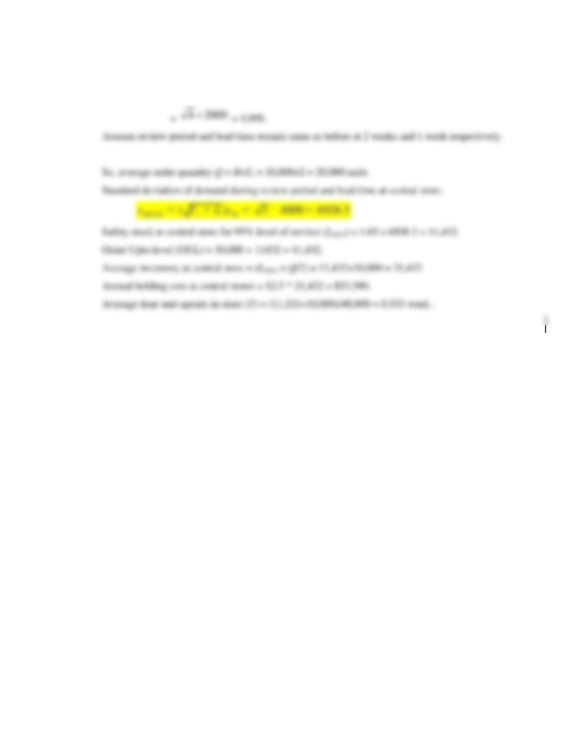
Standard deviation of demand during lead time at central store ()