Design for Quality and Product Excellence 21
9. A team was formed to study the auto part at Adams Metal Fabricating described in
Problem 8. While continuing to work to find the root cause of scrap, the team found a way to
reduce the cost for scrapping the part to $45 per part.
a. Determine the Taguchi loss function for this situation.
b. If customer complaints peak when the parts are more than 2.20 centimeters (cm) above or
below the nominal dimension, what is the loss?
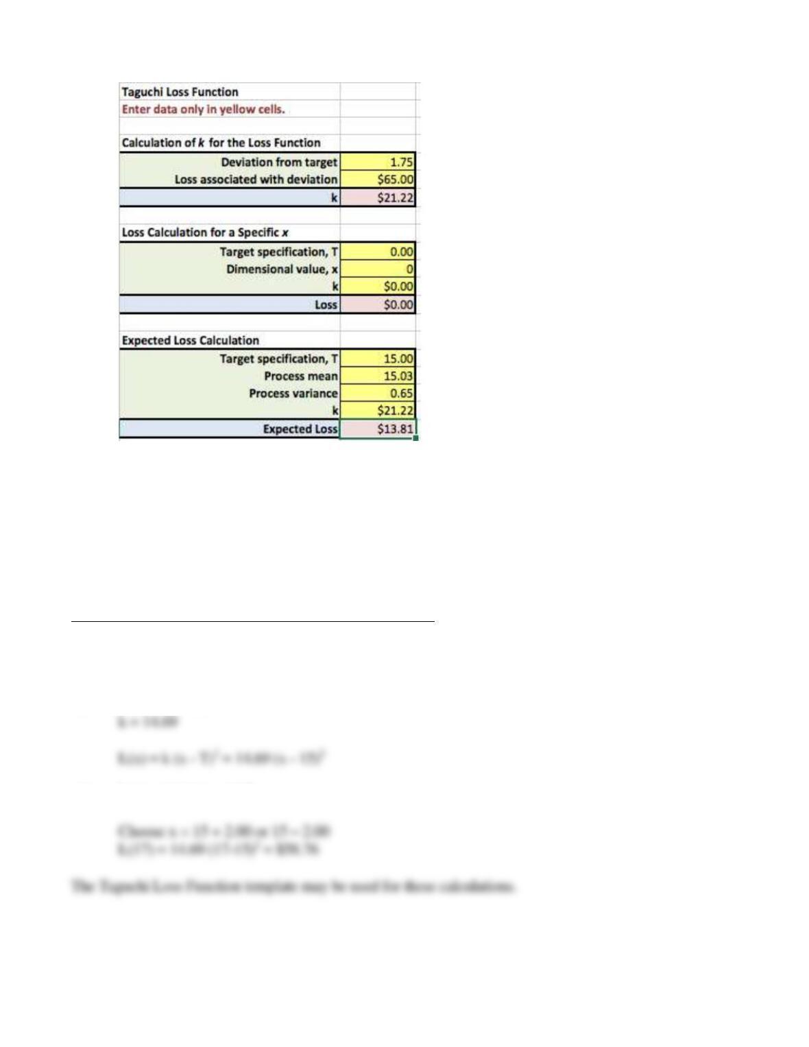
See the Excel file Problem 7.9 in the instructor materials.
The Taguchi Loss Function is: L(x) = k (x – 15)2
a) $45 = k (1.75) 2
b) L(x) = 14.69 (x – 15)2
Design for Quality and Product Excellence 22
10. Ruido Unlimited makes electronic soundboards for car stereos. Output voltage to a certain
component on the board must be 12 ± 0.5 volts. Exceeding the limits results in an estimated
loss of $60. Determine the Taguchi loss function.
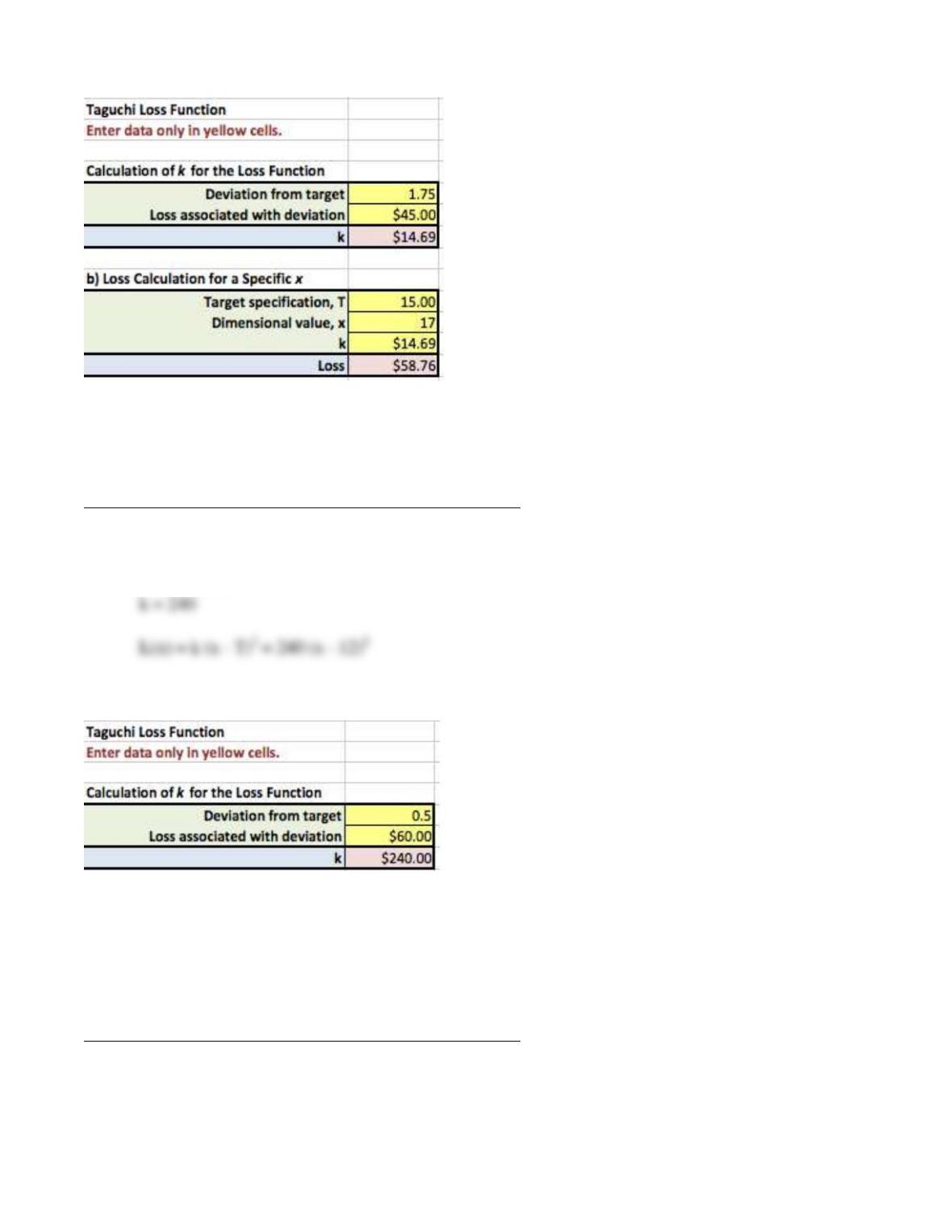
See the Excel file Problem 7.10 in the instructor materials.
The Taguchi Loss Function is: L(x) = k (x – T)2
$60 = k (0.5)2
The Taguchi Loss Function template may be used for these calculations.
11. An electronic component at Ampcomp has a specification of 100 ± 0.4 ohms. Scrapping the
component results in a $81 loss.
a. What is the value of k in the Taguchi loss function?
b. If the process at Ampcomp averages 99.75 ohms with a standard deviation of 0.2 ohms, what
is the expected loss per unit?
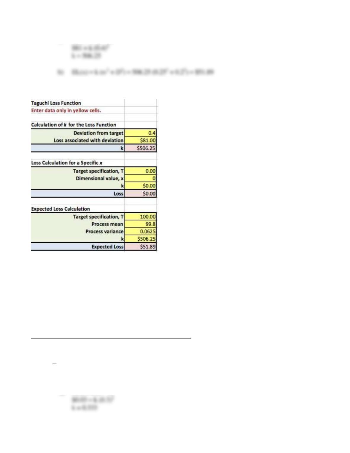
See the Excel file Problem 7.11 in the instructor materials.
For Ampcomp’s specification of 100 ± 0.4 ohms:
Design for Quality and Product Excellence 23
a) L(x) = k (x – T)2
The Taguchi Loss Function template may be used for these calculations.
12. An automatic cookie machine at ACM, Inc., must deposit a specified amount of 25 ± 0.3
grams (g) of dough for each cookie on a conveyor belt. It costs $0.03 to scrap a defective
cookie. A sample of 50 cookies was drawn from the production process, which has been
determined to be approximately normally distributed, and the results, in grams, can be found
in the C07 Problem Data workbook.
a. What is the value of k in the Taguchi loss function?
b. Determine how much the process varies from the target specification, based on the mean
difference and standard deviation of the sample results. What is the expected loss per unit?
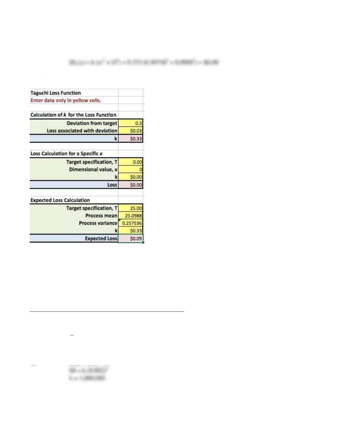
See the Excel file Problem 7.12 in the instructor materials.
Analysis of the dataset provides the following statistics:
x
= 25.0988; D = 25.0988 – 25.0000 = 0.0988
= 0.50748
a) L(x) = k (x – T)2
Design for Quality and Product Excellence 24
b) For = 0.50748
The Taguchi Loss Function template may be used for these calculations.
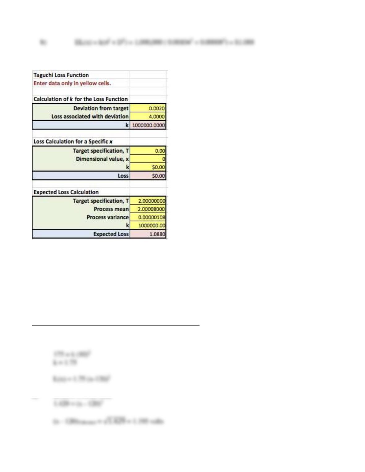
13. A computer chip designed by the MicroKeeb Co. has a specification for the distance
between two adjacent pins of 2.000 ± 0.002 mm. The loss due to a defective chip is $4. A sample
of 25 chips was drawn from the production process and the results, in millimeters, can be
found in the worksheet tab Prob. 7-13 in the Excel file C07Data.
a. Compute the value of k in the Taguchi loss function.
b. What is the expected loss from this process based on the sample data?
See the Excel file Problem 7.13 in the instructor materials.
Analysis of the dataset provides the following statistics:
x
= 2.00008; D = 2.00008 – 2.00 = 0.00008
= 0.00104
Design for Quality and Product Excellence 25
The Taguchi Loss Function template may be used for these calculations.
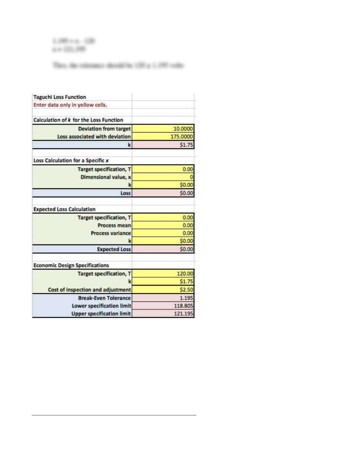
14. In the production of Rembrandt Transformers, any output voltage that exceeds 120 ± 10
volts is unacceptable to the customer. Exceeding these limits results in an estimated loss of
$175. However, the manufacturer can adjust the voltage in the plant by changing a resistor
that costs $2.50.
a. Determine the Taguchi loss function.
b. Suppose the nominal specification is 120 volts. At what tolerance should the transformer be
manufactured, assuming that the amount of loss is represented by the cost of the resistor?
See the Excel file Problem 7.14 in the instructor materials.
a) The Taguchi Loss function is: L(x) = k (x – T)2
Design for Quality and Product Excellence 26
The Taguchi Loss Function template may be used for these calculations.
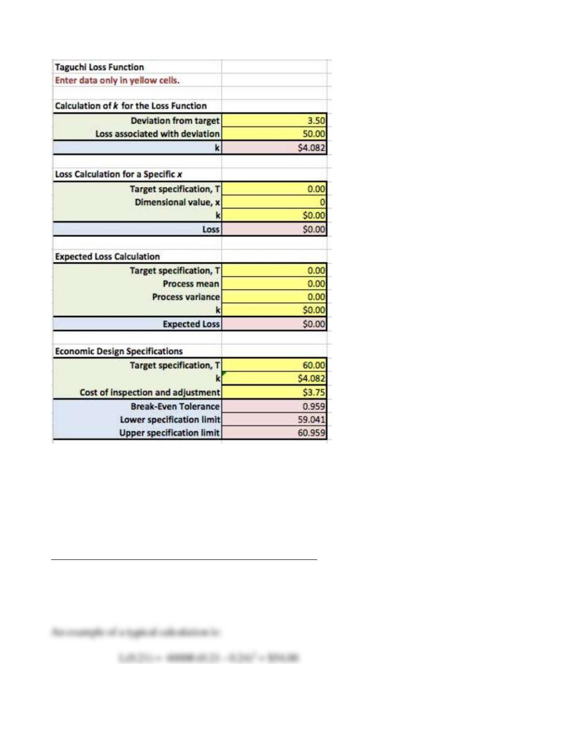
15. At Elproparts Manufacturers’ integrated circuit business, managers gathered data from a
customer focus group and found that any output voltage that exceeds 60 ± 3.5 volts was
unacceptable to the customer. Exceeding these limits results in an estimated loss of $90.
However, the manufacturer can still adjust the voltage in the plant by changing a resistor that
costs $3.75.
a. Determine the Taguchi loss function.
b. Suppose the nominal specification remains at 60 volts. At what tolerance should the
integrated circuit be manufactured, assuming that the amount of loss is represented by the cost
of the resistor?
See the Excel file Problem 7.15 in the instructor materials.
Design for Quality and Product Excellence 27
a) The Taguchi Loss function is: L(x) = k (x – T) 2
50 = k (3.5)2
b) The Taguchi Loss function is: L(x) = k (x – T) 2
$3.75 = 4.082 (x–60)2
0.9187 = (x – 60)2
The Taguchi Loss Function template may be used for these calculations.
Design for Quality and Product Excellence 28
16. Two processes, P and Q, are used by a supplier to produce the same component, Z, which
is a critical part in the engine of the BearingPort 778 airplane. The specification for Z calls for
a dimension of 0.24 mm ± 0.03. The probabilities of achieving the dimensions for each process
based on their inherent variability are provided in the C07 Problem Data workbook. If k =
60,000, what is the expected loss for each process? Which would be the best process to use,
based on minimizing the expected loss?
See the Excel file Problem 7.16 in the instructor materials.
Specifications are 0.24 ± 0.03 mm
L(x) = 60000 (x – .24)2
Design for Quality and Product Excellence 29
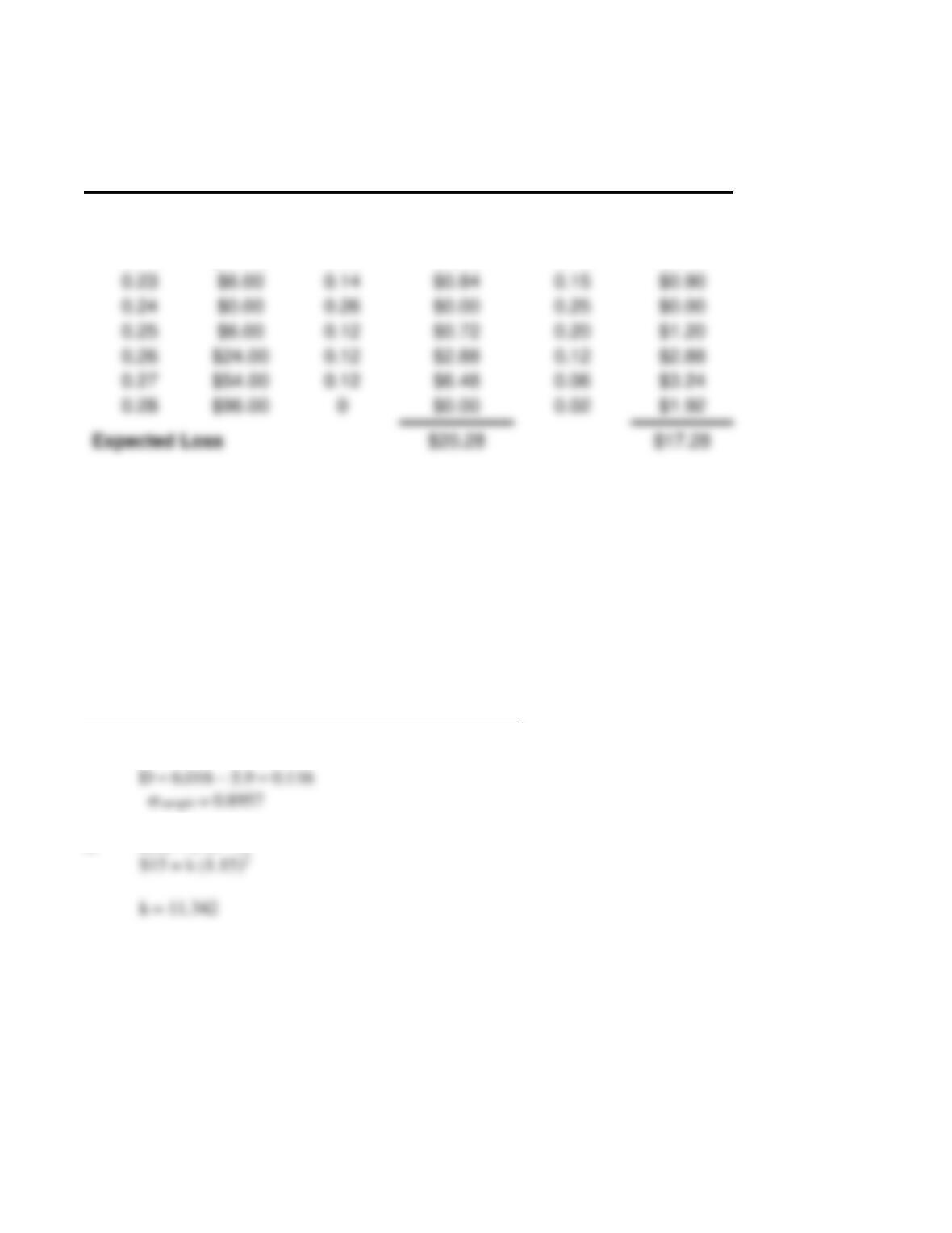
The weighted losses and expected values are shown below:
Value
Loss ($)
Process P
Probability
Weighted
Loss ($)
Process Q
Probability
Weighted
Loss ($)
0.20
$96.00
0
$0.00
0.02
$1.92
0.21
$54.00
0.12
$6.48
0.03
$1.62
0.22
$24.00
0.12
$2.88
0.15
$3.60
Therefore, Process Q incurs a smaller loss than Process P, even though some output of Q falls
outside specifications.
17. The average time to handle a call in the Call-Nowait call processing center has a
specification of 5.9 1.15 minutes. The loss due to a mishandled call is $15. A sample of 25
calls was drawn from the process and the results, in minutes, can be found in the C07 Problem
Data workbook.
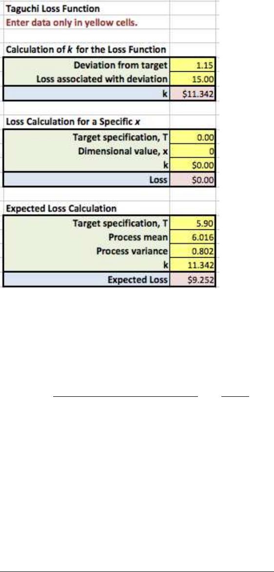
a. Compute the value of k in the Taguchi loss function.
b. What is the expected loss from this process based on the sample data?
See the Excel file Problem 7.17 in the instructor materials.
x = 6.016
a) L(x) = k (x – T)2
b) EL(x) = k ( 2 + D2) = 11.342 (0.89572 + 0.1162) = $9.252
The Taguchi Loss Function template may be used for these calculations.
0.24
0.26
$0.00
0.25
$0.00
0.25
0.12
$0.72
0.20
$1.20
0.27
$54.00
0.12
$6.48
0.06
$3.24
Design for Quality and Product Excellence 30
18. Massive Corporation tested five motors in a 900-hour test. Compute the failure rate if three
failed after 200, 475, and 750 hours and the other two ran for the full 900 hours each.
Massive Corporation’s motors have a failure rate of:
= 3 = 3 = 0.00093 failures / hour
[(2 x 900) + 200 +475 + 750] 3225
19. The life of a Cellurific phone battery is normally distributed with a mean of 1,100 days
and standard deviation of 60 days. Using Excel functions (see Chapter 6), determine the
following:
a. What fraction of batteries is expected to survive beyond 1,200 days?
b. What fraction will survive fewer than 995 days?
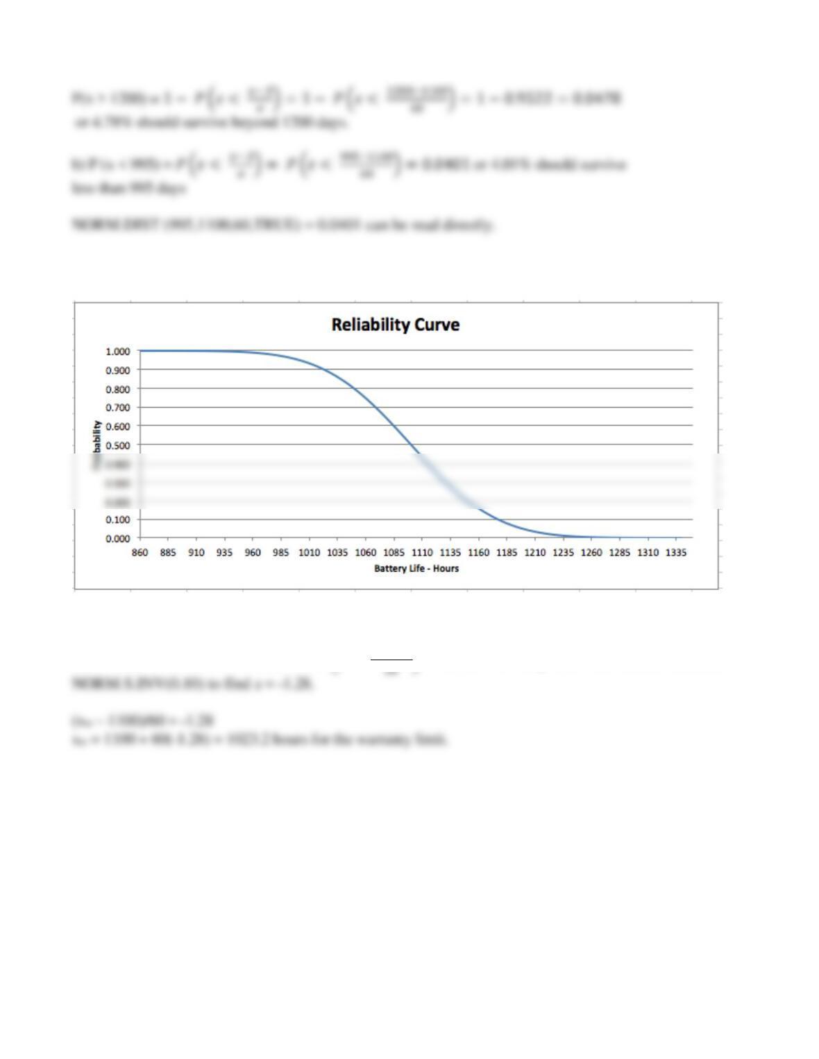
c. Draw a chart of the reliability function using Excel.
d. What length of warranty is needed so that no more than 10 percent of the batteries will be
expected to fail during the warranty period?
See the Excel file Problem 7.19 in the instructor materials.
a) P(x > 1200) = 1 – P(x < 1200)
Using the Excel NORM.DIST (1200,1100,60,TRUE) = 0.9522
Design for Quality and Product Excellence 31
c) The reliability function looks approximately as follows:
d) Let xw be the limit of the warranty period.
P(x < xw) = 0.10; z = -1.28, for 𝑃 (𝑧 = 𝑥−1100
20. Broadtred, Inc. makes automobile tires that have a mean life of 50,000 miles with a
standard deviation of 2,500 miles. Using Excel functions (see Chapter 6), determine the
following:
a. What fraction of tires is expected to survive beyond 54,000 miles?
b. What fraction will survive fewer than 56,000 miles?
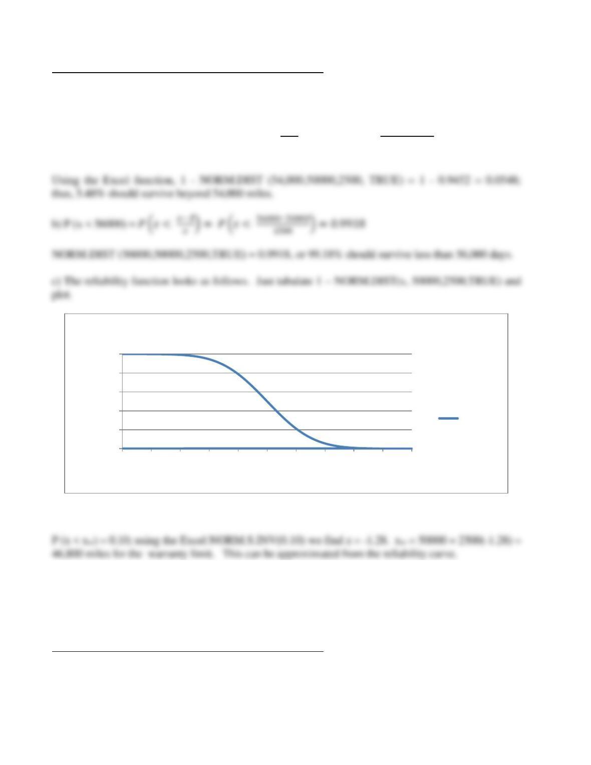
c. Draw a chart of the reliability function using Excel.
d. What length of warranty is needed so that no more than 2 percent of the tires will be
expected to fail during the warranty period?
Design for Quality and Product Excellence 32
See the Excel file Problem 7.20 in the instructor materials.
a) P(x > 54,000) = 1 – P(x < 54,000)
Analytically, P(x > 54000) = 1 − 𝑃 (𝑧 < 𝑥− 𝑥̅
𝜎) = 1 − 𝑃(𝑧 < 54000−50000
2500 ) = 1 − 0.9452 =
0.0548
d) Let xw be the limit of the warranty period.
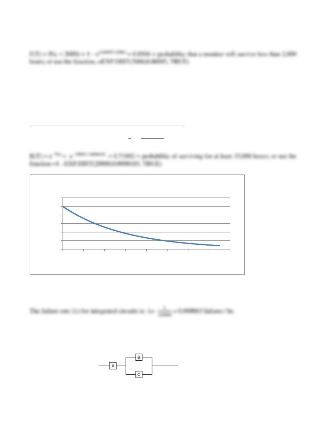
21. Livelong, Inc.’s computer monitors have a failure rate of 0.00095 units per hour. What is
the reliability function? Assuming an exponential distribution, what is the probability of
failure within 5,000 hours? Calculate your answer using the appropriate mathematical
formula and verify your result using Excel.
See the Excel file Problem 7.21 in the instructor materials.
The reliability function is R(T) = 1 – F(T) = e–T = e –0.00095T
0.000
0.200
0.400
0.600
0.800
1.000
40000 42000 44000 46000 48000 50000 52000 54000 56000 58000 60000
Probability
Tread Life – Miles
Reliability Curve
Reliability
Design for Quality and Product Excellence 33
= 0.00095; use F(2000) = P(x < 2000)
22. An electronic component in a satellite radio made by Spacescope, Inc. has failure rate of
= 0.0000165. Find the mean time to failure (MTTF). What is the probability (assuming an
exponential probability distribution) that the component will not have failed after 20,000 hours
of operation? Calculate your answer using the appropriate mathematical formula and verify
your result using Excel. Then draw the reliability function to verify your answer visually.
See the Excel file Problem 7.22 in the instructor materials.
The MTTF for the component is 𝜃 = 1
𝜆= 1
0.0000165; so, = 60606.06
23. The MTBF of an integrated circuit made by Wayforward, Inc. is 16,000 hours. Calculate
the failure rate.
24. A manufacturer of electric cooktops purchases major electronic components as modules.
The reliabilities of components differ by supplier (see diagram, below). Suppose that the
configuration of the major components is given by:
0.000
0.200
0.400
0.600
0.800
1.000
1.200
0 20000 40000 60000 80000 100000 120000 140000 160000
Probability
Hours to Failure
Reliability Function