Markov Processes
Chapter 7
An Introduction to Linear Programming
Learning Objectives
1. Obtain an overview of the kinds of problems linear programming has been used to solve.
5. Understand the importance of extreme points in obtaining the optimal solution.
6. Know the use and interpretation of slack and surplus variables.
7. Be able to interpret the computer solution of a linear programming problem.
8. Understand how alternative optimal solutions, infeasibility and unboundedness can occur in linear
programming problems.
Chapter 17
Solutions:
1. a, b, and e, are acceptable linear programming relationships.
c is not acceptable because of
2
2B−
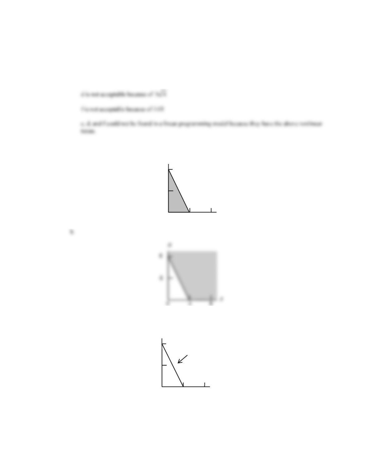
2. a.
8
4
4
8
0
B
A
c.
B
A
8
4
4
8
0
Points on line
are only feasible
points
Markov Processes
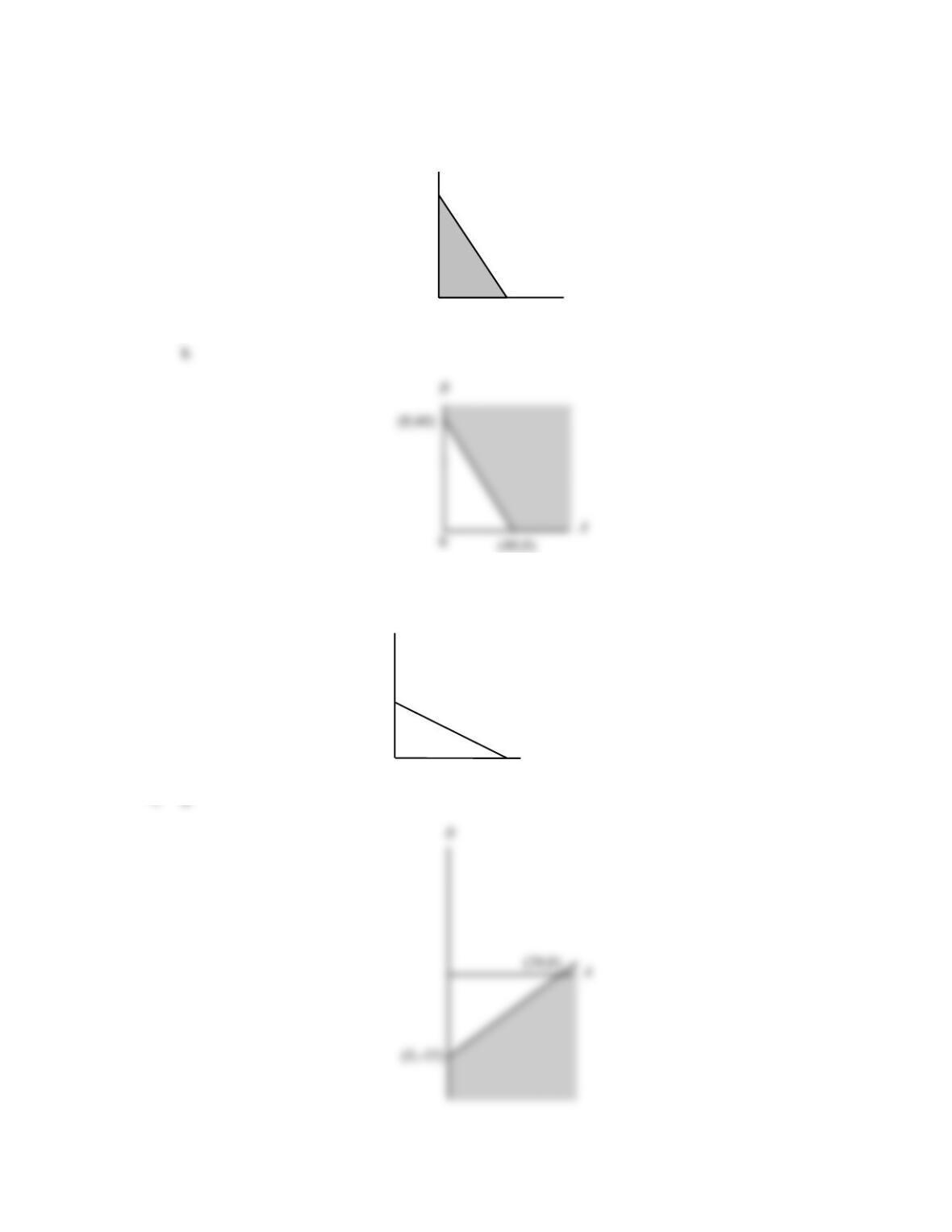
3. a.
B
A
0
(0,9)
(6,0)
c.
B
A
0
(0,20)
(40,0)
Points
on line are only
feasible solutions
Chapter 17
c.
B
A
0
(10,25)
Note: Point shown was
used to locate position of
the constraint line
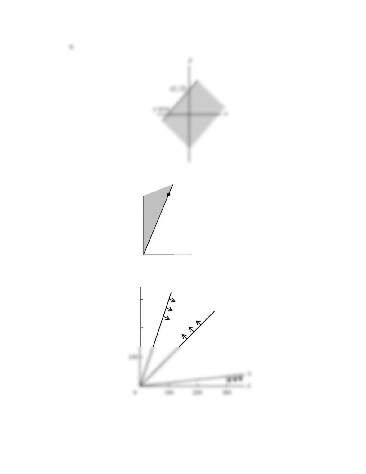
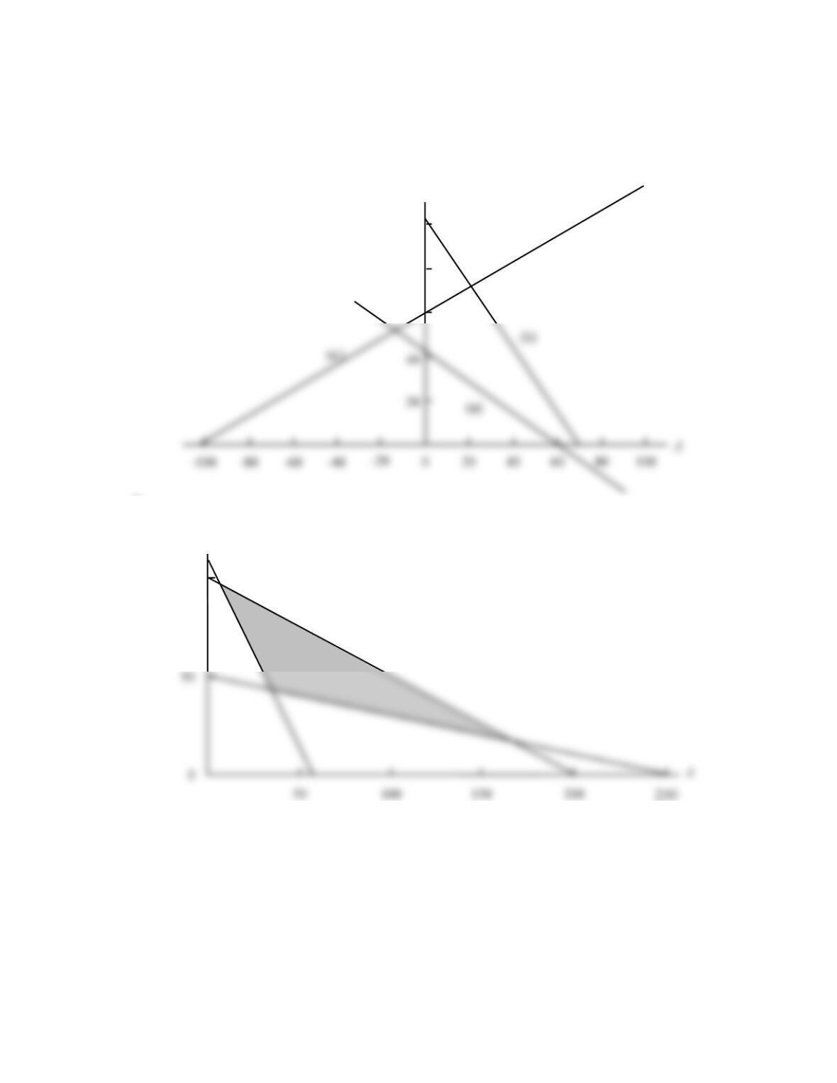
5.
B
100
200
300
a
c
Markov Processes
6. a. 7A + 10B = 420
b. 6A + 4B = 420
c. -4A + 7B = 420
80
40
40
80
20
20
60
100
B
60
100
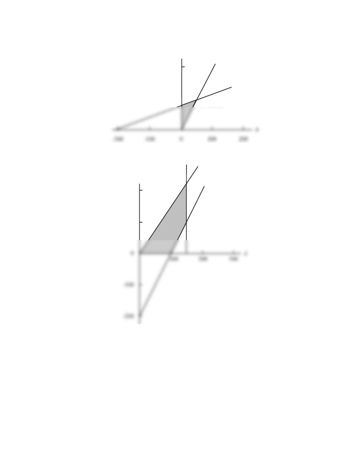
7.
50
B
100
Chapter 17
8.
200
133
1
/
3
(100,200)
B
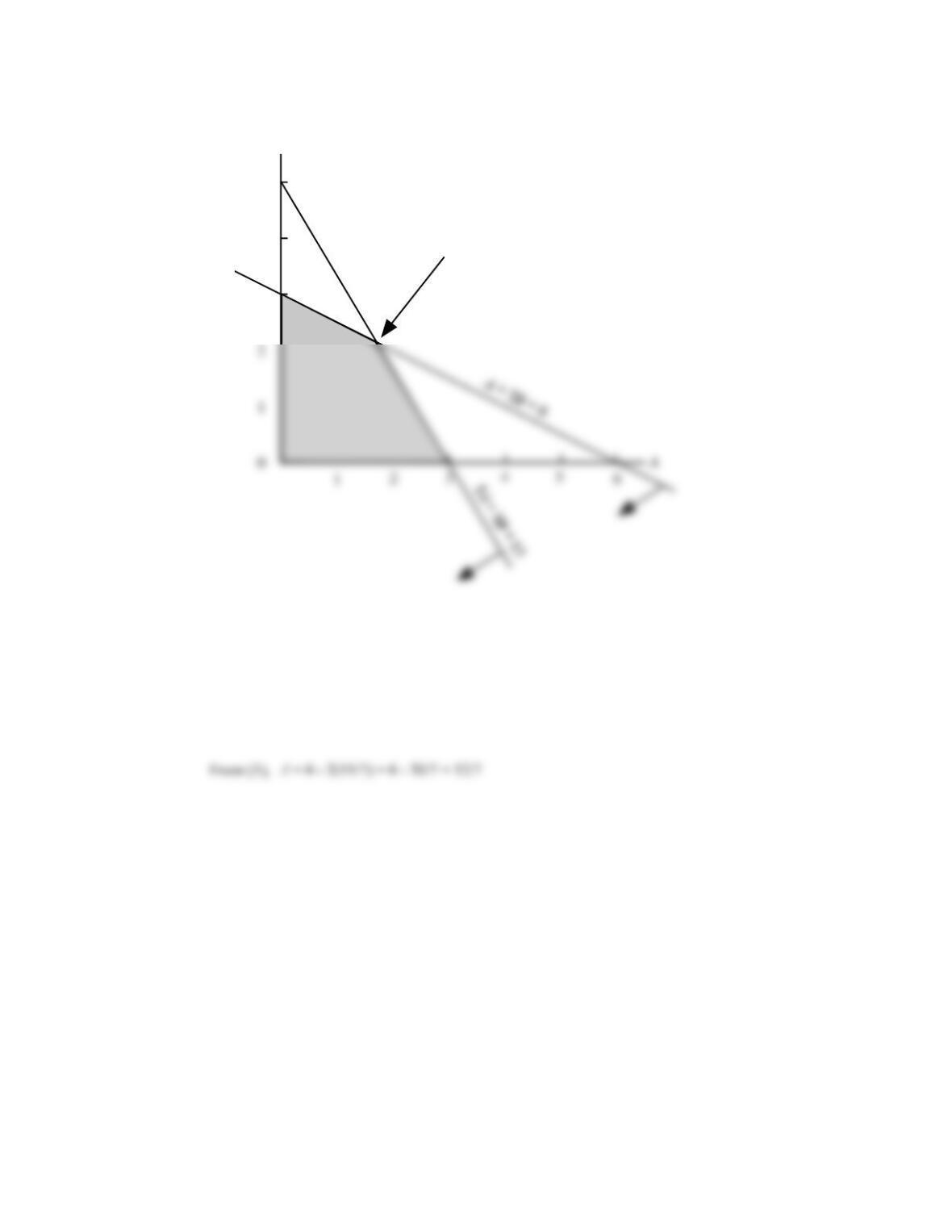
9.
B
A
200
100
(150,225)
(150,100)
Markov Processes
10.
3
4
5
B
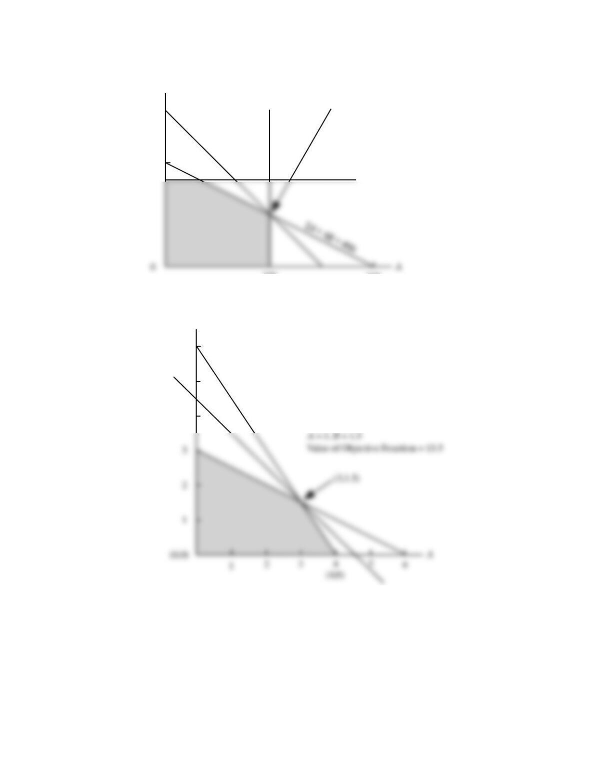
Optimal Solution
A= 12/7, B= 15/7
Value of Objective Function = 2(12/7) + 3(15/7) = 69/7
A
+
2B
=
6
(1)
5A
+
3B
=
15
(2)
(1) × 5
5A
+
10B
=
30
(3)
(2) – (3)
–
7B
=
–15
B
=
15/7
Chapter 17
11.
100
B
100 200
Optimal Solution
A= 100, B= 50
Value of Objective Function = 750
A= 100
B= 80
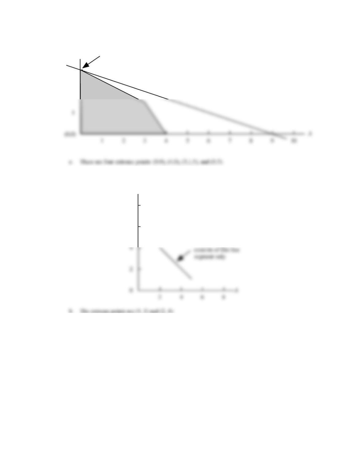
12. a.
4
5
B
Optimal Solution
6
Markov Processes
b.
2
3
B
Optimal Solution
A= 0, B= 3
Value of Objective Function = 18
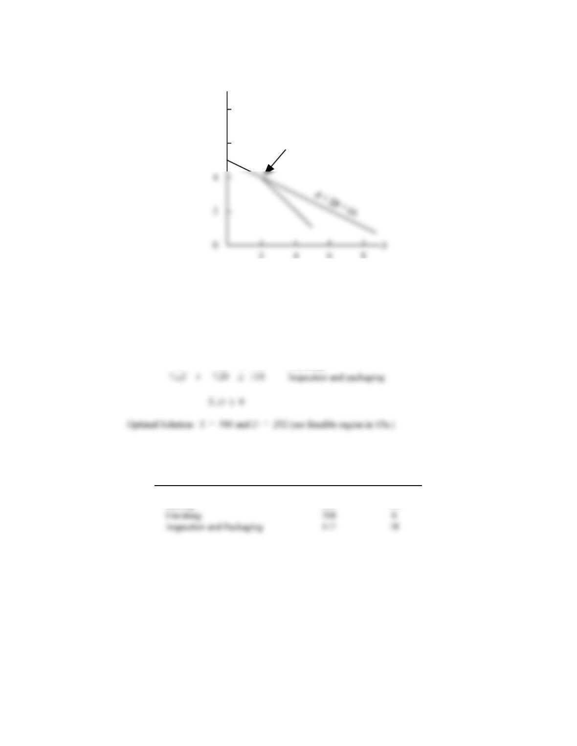
13. a.
6
8
B
Feasible Region
Chapter 17
c.
6
8
B
2 4 6 8
Optimal Solution
A= 2, B= 4
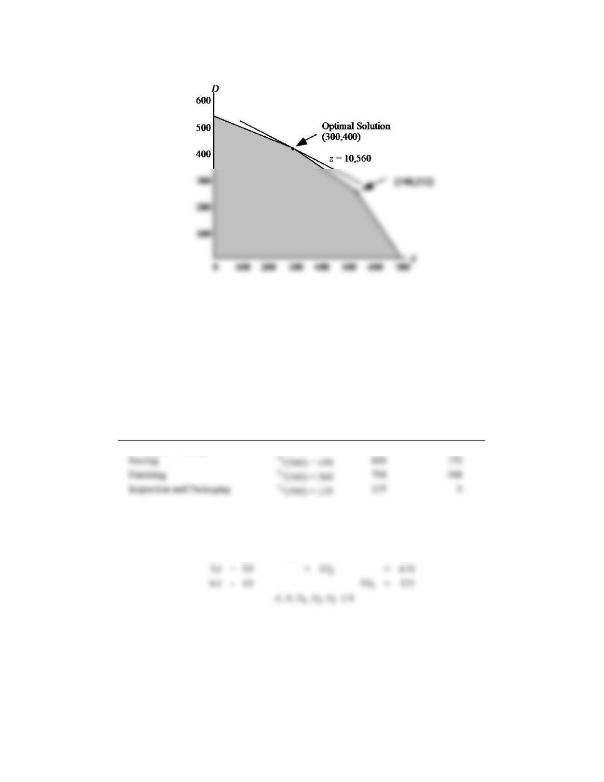
14. a. Let S = number of standard bags
D = number of deluxe bags
Max
10S
+
9D
s.t.
7/10S
+
1D
630
Cutting and dyeing
1/2 S
+
5/6D
600
Sewing
1/10S
+
1/4D
135
Inspection and packaging
1S
+
2/3D
708
Finishing
b. Profit = $7668
c. & d.
Department
Production Time
Slack
Cutting and Dyeing
630
0
Sewing
480
120
Finishing
708
0
Inspection and Packaging
117
Markov Processes
15. a.
b. Similar to part (a): the same feasible region with a different objective function. The optimal
solution occurs at (708, 0) with a profit of z = 20(708) + 9(0) = 14,160.
c. The sewing constraint is redundant. Such a change would not change the optimal solution to the
original problem.
16. a. A variety of objective functions with a slope greater than -4/10 (slope of I & P line) will make
extreme point (0, 540) the optimal solution. For example, one possibility is 3S + 9D.
b. Optimal Solution is S = 0 and D = 540.
c.
Department
Hours Used
Max. Available
Slack
Cutting and Dyeing
1(540) = 540
630
90
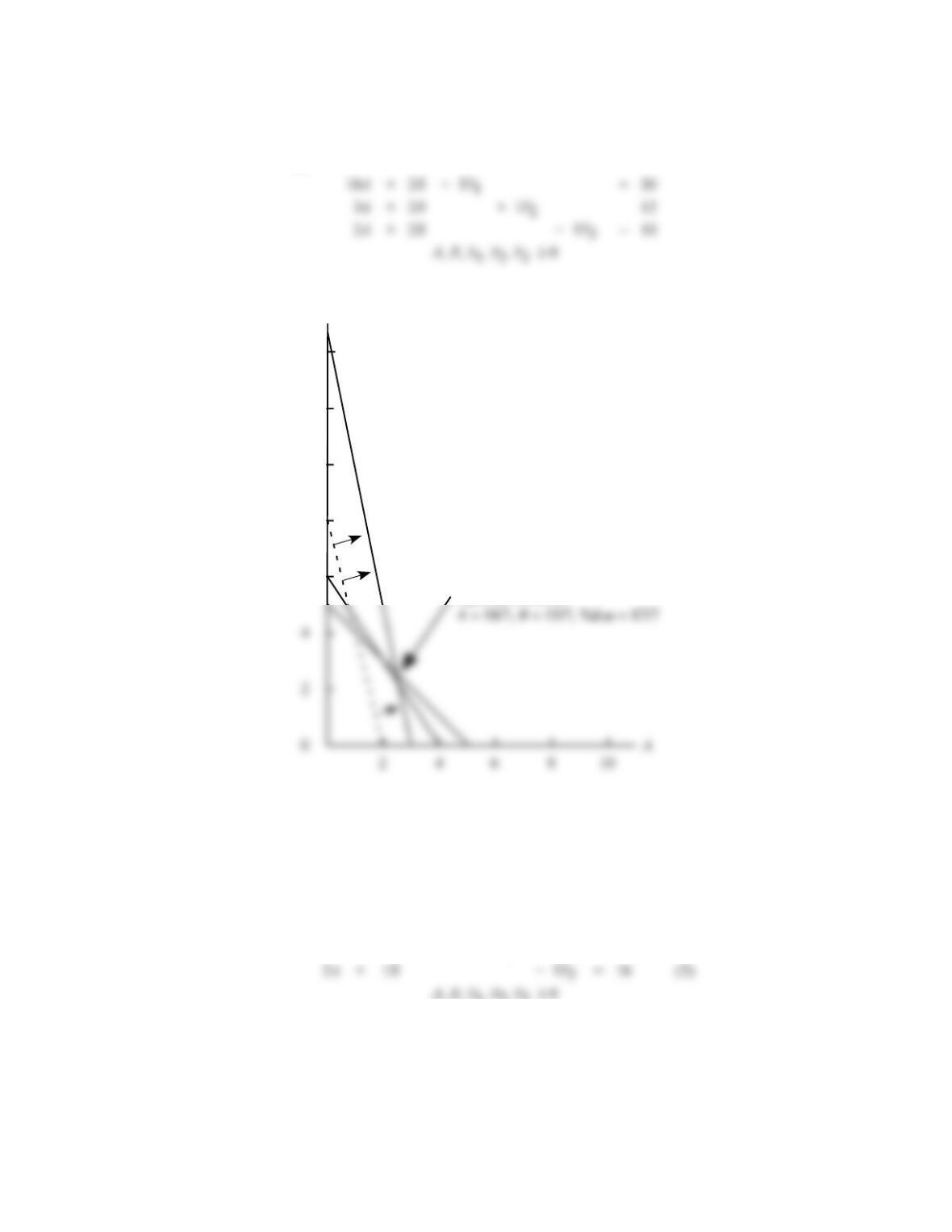
17.
Max
5A
+
2B
+
0S1
+
0S2
+
0S3
s.t.
2A
+
3B
+
1S2
=
610
1S3
1A
–
2B
+
1S1
=
420
Chapter 17
18. a.
Max
4A
+
1B
+
0S1
+
0S2
+
0S3
s.t.
+
+
1S1
=
3A
+
2B
+
1S2
=
2A
+
2B
+
1S3
=
b.
6
8
B
10
12
14
c. S1 = 0, S2 = 0, S3 = 4/7
19. a.
Max
3A
+
4B
+
0S1
+
0S2
+
0S3
s.t.
-1A
+
2B
+
1S1
=
8 (1)
1A
+
2B
+
1S2
=
12 (2)
2A
+
1B
+
1S3
=
16 (3)
Markov Processes
b.
0
B
2 4 6 8
A
10
12
14
10 12
(2)
(1)
(3)
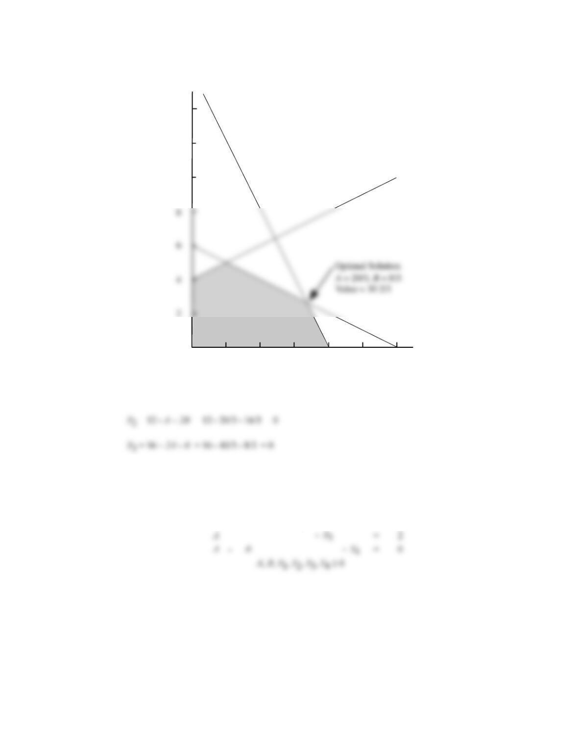
c. S1 = 8 + A – 2B = 8 + 20/3 – 16/3 = 28/3
20. a.
Max
3A
+
2B
s.t.
A
+
B
– S1
=
4
3A
+
4B
+ S2
=
24
=
2
–
B
=
0
Chapter 17
b.
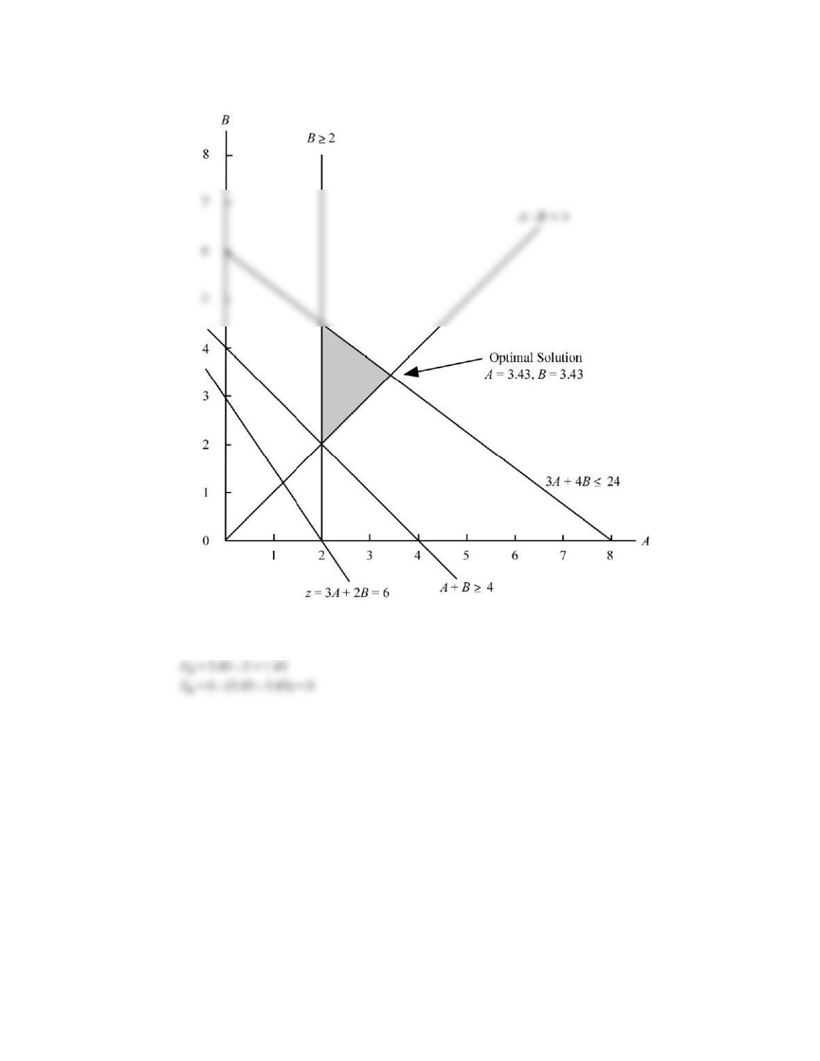
c. S1 = (3.43 + 3.43) – 4 = 2.86
S2 = 24 – [3(3.43) + 4(3.43)] = 0
Markov Processes
21. a. and b.
B
Optimal Solution
50
60
70
80
90
Constraint 2
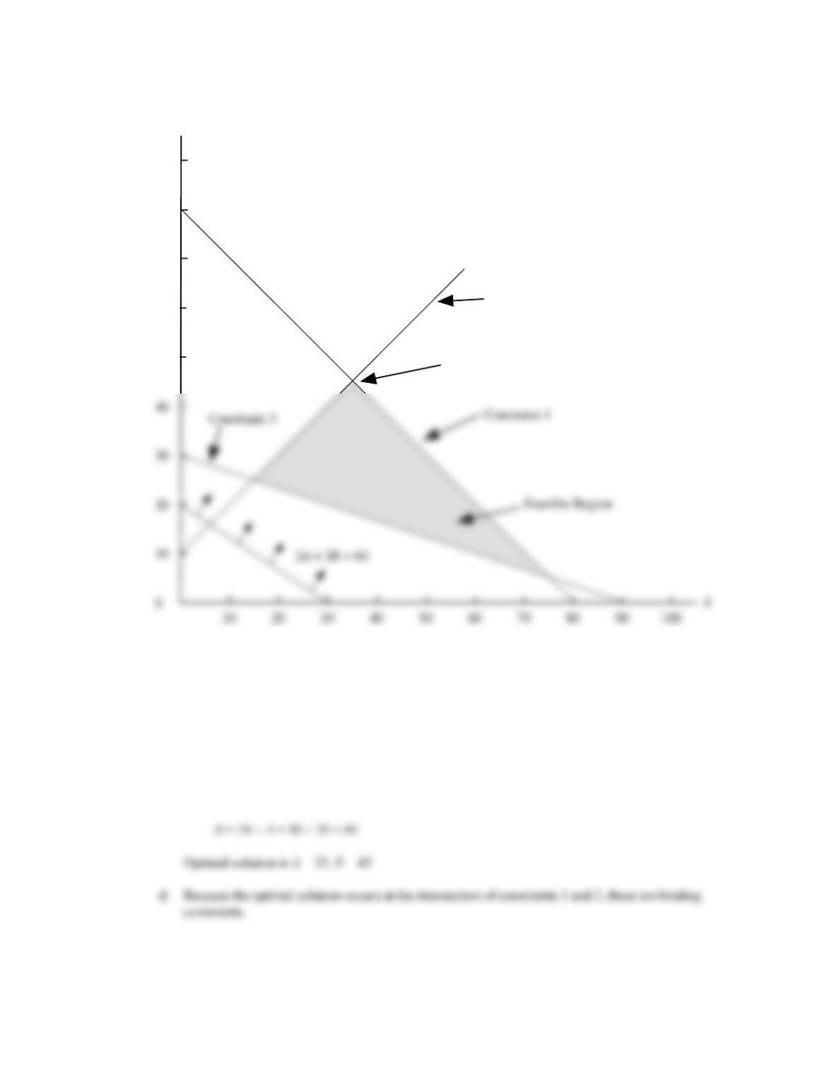
c. Optimal solution occurs at the intersection of constraints 1 and 2. For constraint 2,
B = 10 + A
Substituting for B in constraint 1 we obtain
5A + 5(10 + A)
= 400
5A + 50 + 5A
= 400
10A
= 350
A
= 35
Chapter 17
22. a.
2000
C
2500
3000
3500
Inspection and
Packaging
Cutting and
Dyeing
5
b.
Extreme Point
Coordinates
Profit
1
(0, 0)
5(0) + 4(0) = 0
2
(1700, 0)
5(1700) + 4(0) = 8500
3
(1400, 600)
5(1400) + 4(600) = 9400
4
(800, 1200)
5(800) + 4(1200) = 8800
5
(0, 1680)
5(0) + 4(1680) = 6720
Extreme point 3 generates the highest profit.
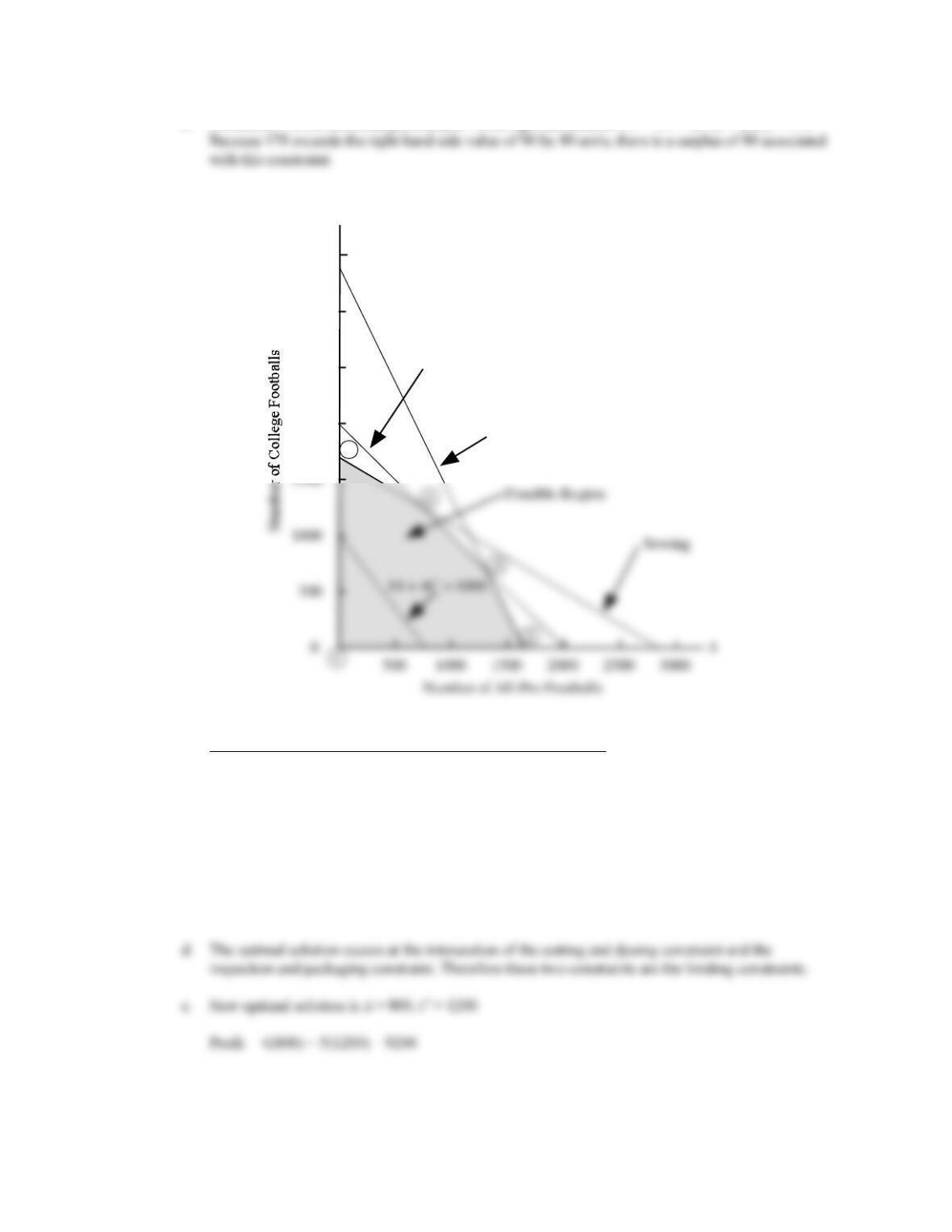
c. Optimal solution is A = 1400, C = 600
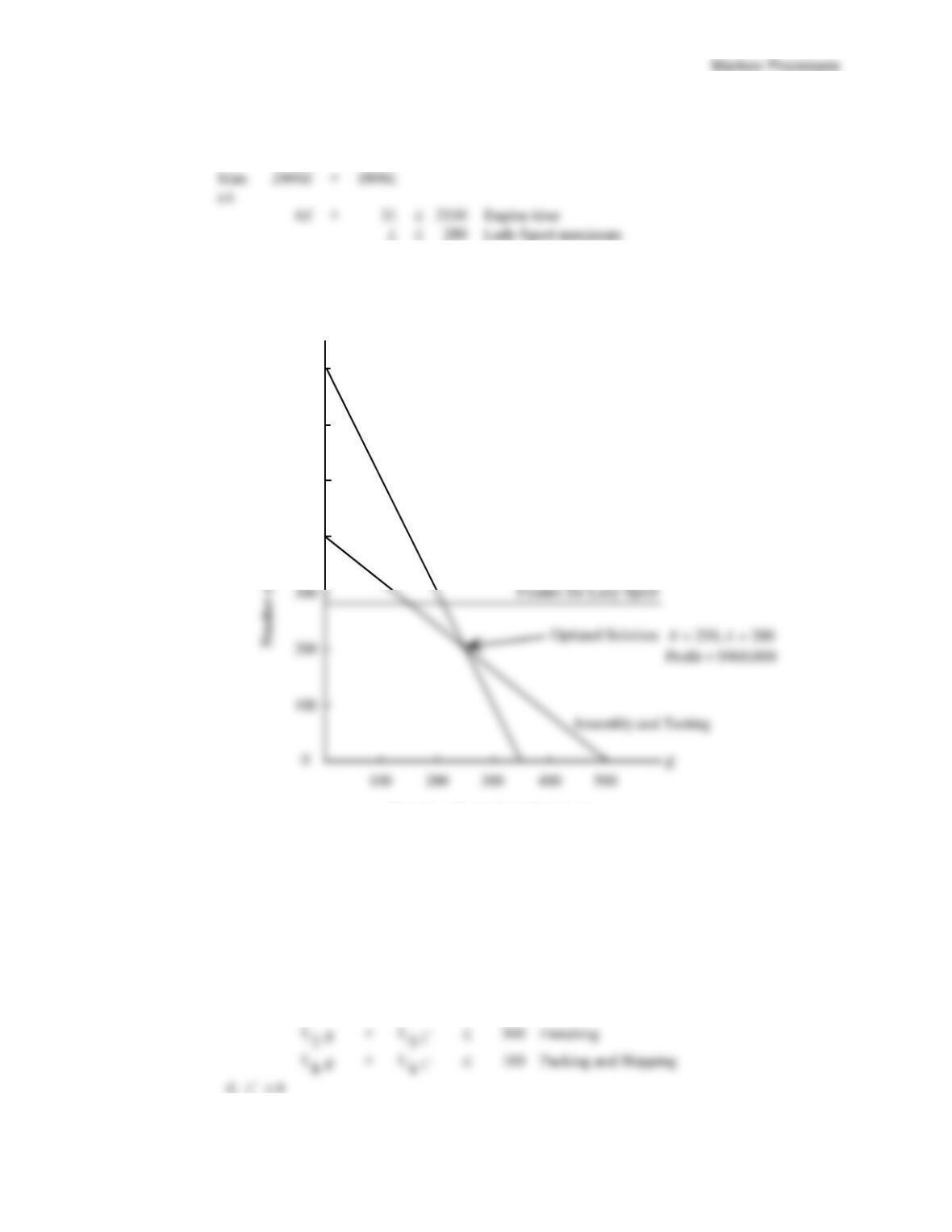
23. a. Let E = number of units of the EZ-Rider produced
L = number of units of the Lady-Sport produced
2E
+
2.5L
1000
Assembly and testing
E, L 0
b.
c. The binding constraints are the manufacturing time and the assembly and testing time.
24. a. Let R = number of units of regular model.
C = number of units of catcher’s model.
Max
5R
+
8C
s.t.
1R
+
3/2 C
900 Cutting and sewing
1/3 C
L
400
500
600
700
Engine
Manufacturing Time
Number of Lady-Sport Produced
Chapter 17
400
400 800
R
200
200 6000 1000
Optimal Solution
(500,150)
P & S
Regular Model
Catcher’s Model
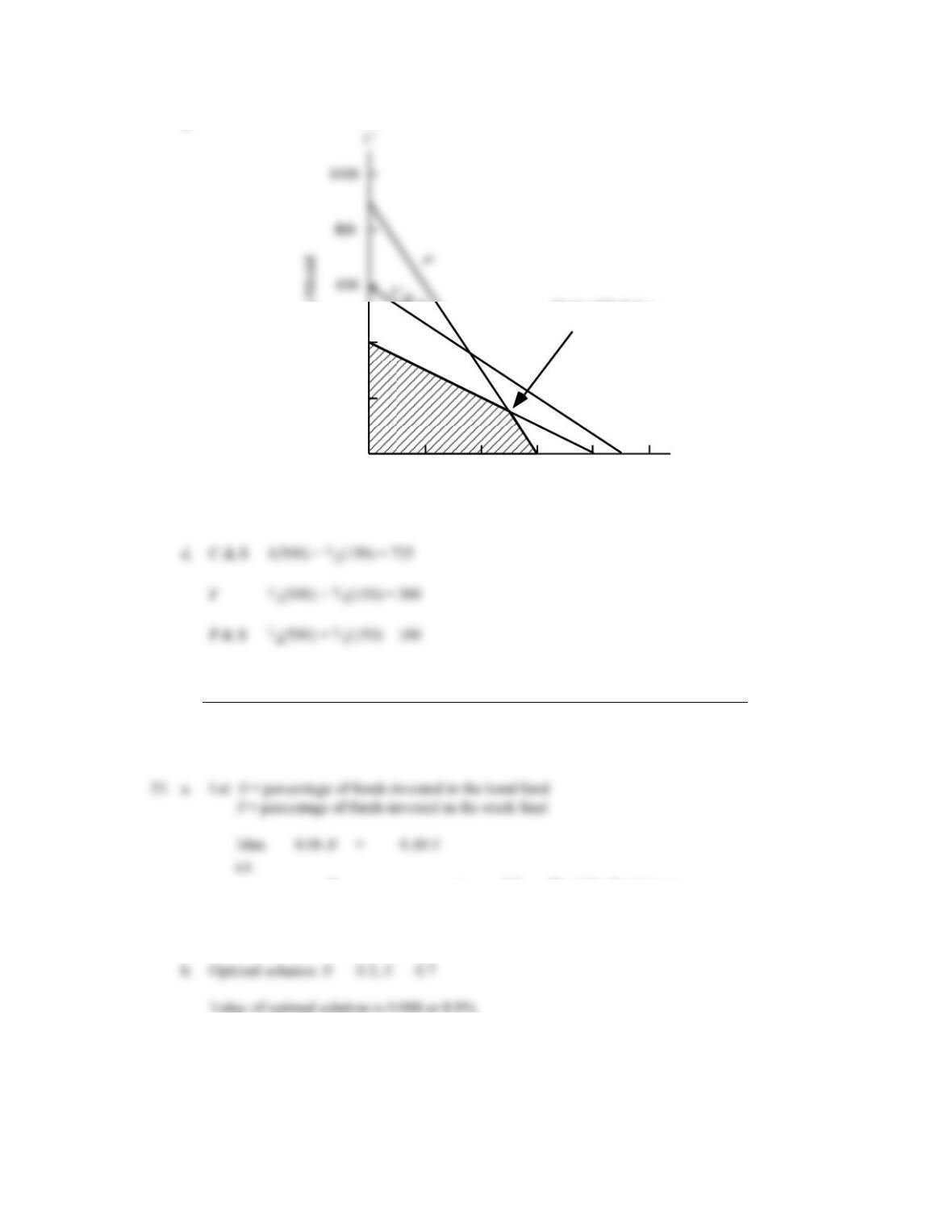
c. 5(500) + 8(150) = $3,700
e.
Department
Capacity
Usage
Slack
C & S
900
725
175 hours
F
300
300
0 hours
P & S
100
100
0 hours
0.06 B
+
0.10 S
s.t.
B
0.3
Bond fund minimum
0.06 B
+
0.10 S
0.075
Minimum return
B
+
S
=
1
Percentage requirement
Markov Processes
26. a. a. Let N = amount spent on newspaper advertising
R = amount spent on radio advertising
Max
50N
+
80R
s.t.
+
-2R
N, R 0
b.
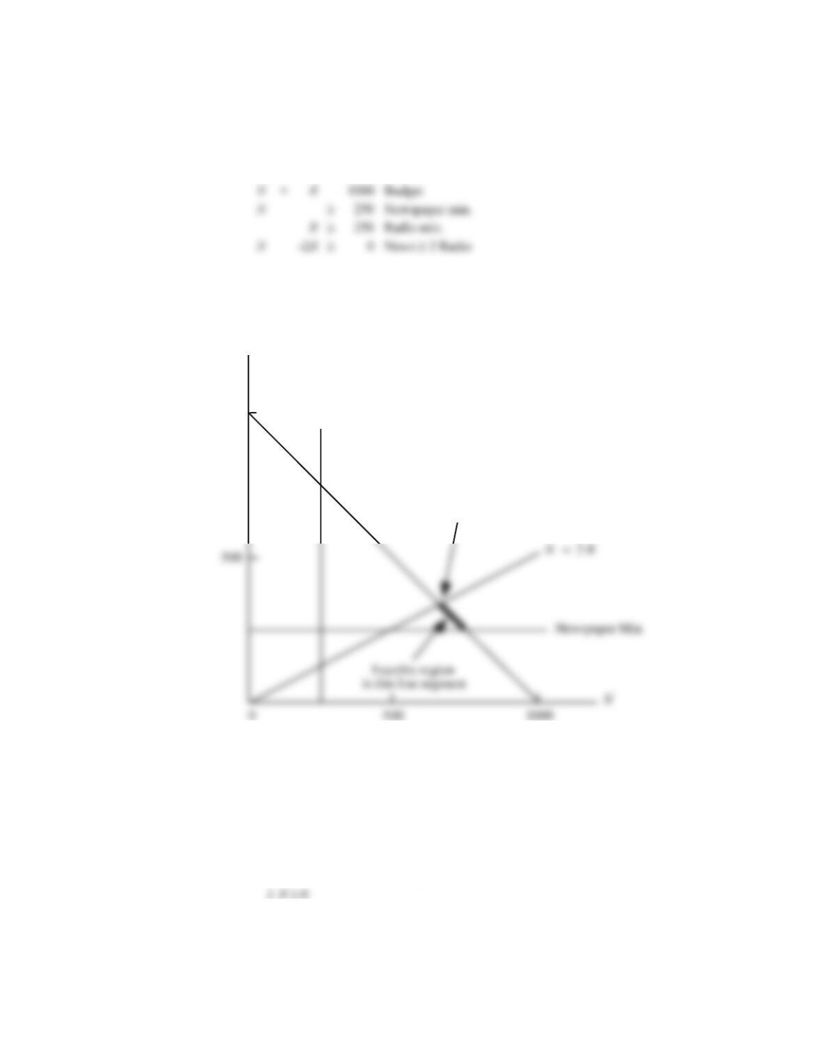
is this line segment
= 2
R
1000
Optimal Solution
N
= 666.67,
R
= 333.33
Value = 60,000
Budget
Radio Min
27. Let I = Internet fund investment in thousands
B = Blue Chip fund investment in thousands
Max
0.12I
+
0.09B
s.t.
1I
+
1B
50
Available investment funds
1I
35
Maximum investment in the internet fund
6I
+
4B
240
Maximum risk for a moderate investor
Chapter 17
Internet fund $20,000
Blue Chip fund $30,000
Annual return $ 5,100
b. The third constraint for the aggressive investor becomes
6I + 4B 320
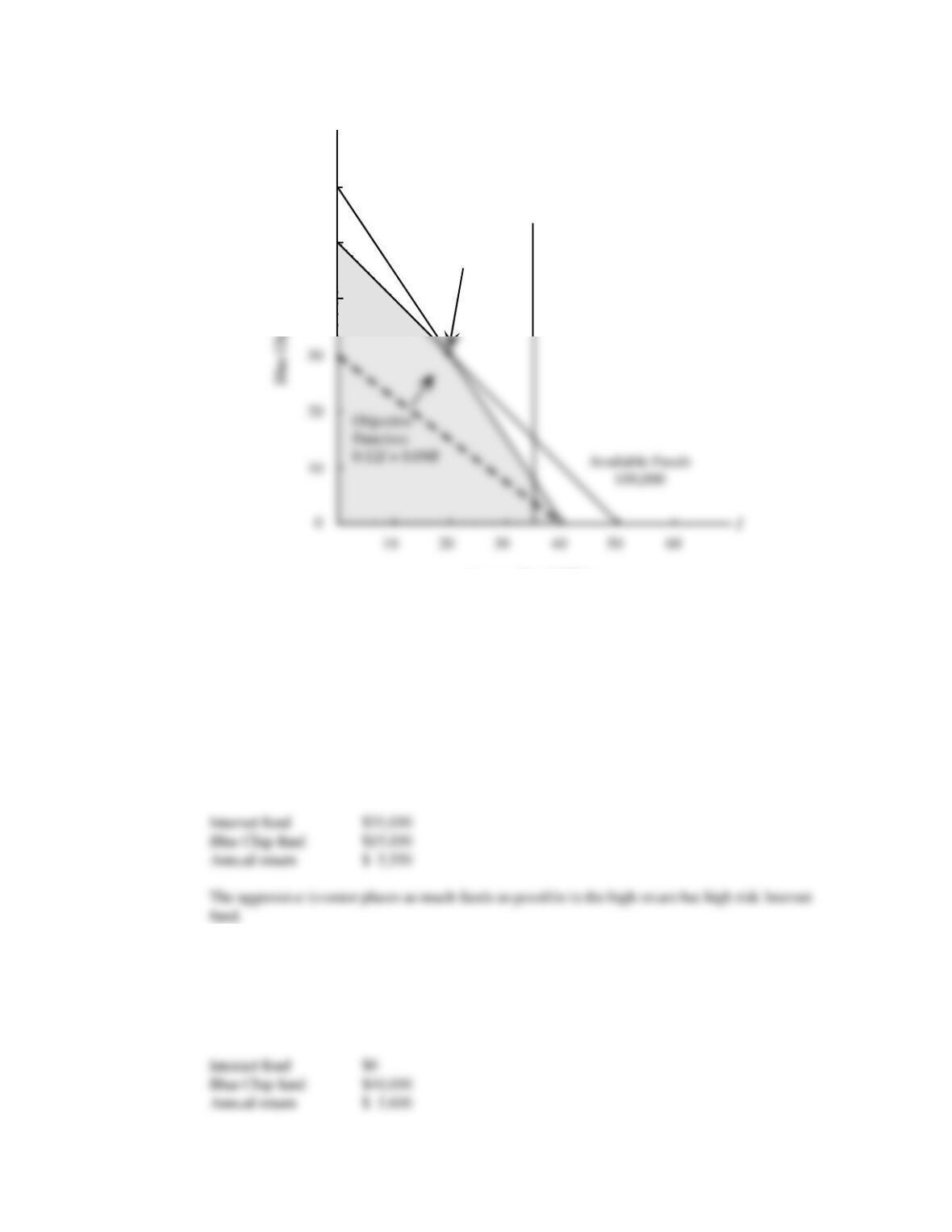
This constraint is redundant; the available funds and the maximum Internet fund investment
constraints define the feasible region. The optimal solution is:
c. The third constraint for the conservative investor becomes
6I + 4B 160
This constraint becomes a binding constraint. The optimal solution is
B
Optimal Solution
40
50
60
Risk Constraint
Maximum
Internet Funds
I = 20, B = 30
$5,100
Internet Fund (000s)