CHAPTER 7
Linear Programming
Models: Graphical and Computer Methods
TEACHING SUGGESTIONS
Teaching Suggestion 7.1: Draw Constraints for a Graphical LP Solution.
Explain constraints of the three types (, = , ) carefully the first time you present an example.
Teaching Suggestion 7.2: Feasible Region Is a Convex Polygon.
Explain Dantzig’s discovery that all feasible regions are convex (bulge outward) polygons
Teaching Suggestion 7.3: Using the Iso-Profit Line Method.
This method can be much more confusing than the corner point approach, but it is faster once
Teaching Suggestion 7.4: QA in Action Boxes in the LP Chapters.
There are a wealth of motivating tales of real-world LP applications in Chapters 7–9. The airline
industry in particular is a major LP user.
Teaching Suggestion 7.5: Feasible Region for the Minimization Problem.
Students often question the open area to the right of the constraints in a minimization problem
Teaching Suggestion 7.6: Infeasibility.
This problem is especially common in large LP formulations since many people will be provid-
ing input constraints to the problem. This is a real-world problem that should be expected.
Teaching Suggestion 7.7: Alternative Optimal Solutions.
This issue is an important one that can be explained in a positive way. Managers appreciate hav-
Teaching Suggestion 7.8: Importance of Sensitivity Analysis.
Sensitivity analysis should be stressed as one of the most important LP issues. (Actually, the is-
sue should arise for discussion with every model). Here, the issue is the source of data. When
ALTERNATIVE EXAMPLES
Alternative Example 7.1: Hal has enough clay to make 24 small vases or 6 large vases. He on-
ly has enough of a special glazing compound to glaze 16 of the small vases or 8 of the large vas-
es. Let X1 = the number of small vases and X2 = the number of large vases. The smaller vases sell
for $3 each, while the larger vases would bring $9 each.
(a) Formulate the problem.
(b) Solve graphically.
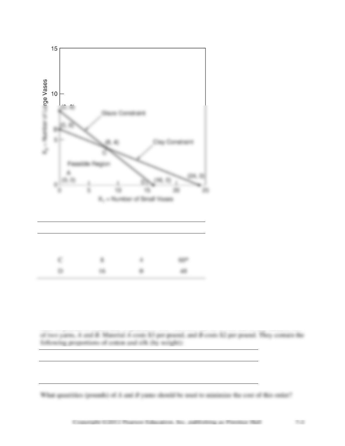
Point
X1
X2
Income
A
0
0
$ 0
B
0
6
54
C
8
4
D
0
48
*Optimum income of $60 will occur by making and selling 8 small vases and 4 large
vases.
Draw an isoprofit line on the graph from (20, 0) to (0, 62/3) as the $60 isoprofit line.
Alternative Example 7.2: A fabric firm has received an order for cloth specified to contain at
least 45 pounds of cotton and 25 pounds of silk. The cloth can be woven out on any suitable mix
Yarn
Cotton (%)
Silk (%)
A
30
50
B
60
10
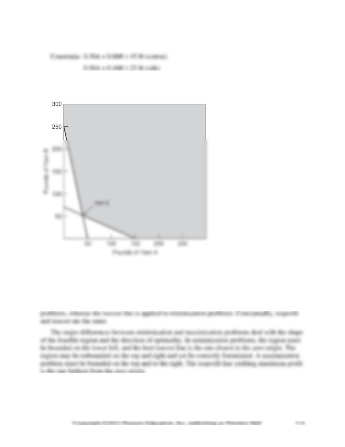
Objective function: min. C = 3A + 2B
Simultaneous solution of the two constraint equations reveals that A = 39 lb, B = 55 lb.
The minimum cost is C = $3A + $2B = 3(39) + (2)(55) = $227.
SOLUTIONS TO DISCUSSION QUESTIONS AND PROBLEMS
7-1. Both minimization and maximization LP problems employ the basic approach of develop-
ing a feasible solution region by graphing each of the constraint lines. They can also both be
solved by applying the corner point method. The isoprofit line method is used for maximization
7-2. The requirements for an LP problem are listed in Section 7.2. It is also assumed that condi-
tions of certainty exist; that is, coefficients in the objective function and constraints are known
with certainty and do not change during the period being studied. Another basic assumption that
7-3. Each LP problem that has a feasible solution does have an infinite number of solutions. On-
7-4. If a maximization problem has many constraints, then it can be very time consuming to use
7-6. This question involves the student using a little originality to develop his or her own LP
constraints that fit the three conditions of (1) unboundedness, (2) infeasibility, and (3) redundan-
cy. These conditions are discussed in Section 7.7, but each student’s graphical displays should be
different.
7-7. The manager’s statement indeed had merit if the manager understood the deterministic na-
ture of linear programming input data. LP assumes that data pertaining to demand, supply, mate-
7-8. The objective function is not linear because it contains the product of X1 and X2, making it a
second-degree term. The first, second, fourth, and sixth constraints are okay as is. The third and
fifth constraints are nonlinear because they contain terms to the second degree and one-half de-
gree, respectively.
7-9. For a discussion of the role and importance of sensitivity analysis in linear programming,
refer to Section 7.8. It is needed especially when values of the technological coefficients and
7-10. If the profit on X is increased from $12 to $15 (which is less than the upper bound), the
same corner point will remain optimal. This means that the values for all variables will not
change from their original values. However, total profit will increase by $3 per unit for every
7-11. If the right-hand side of the constraint is increased from 80 to 81, the maximum total profit
will increase by $3, the amount of the dual price. If the right-hand side is increased by 10 units
(to 90), the maximum possible profit will increase by 10(3) = $30 and will be $600 + $30 =
$630. This $3 increase in profit will result for each unit we increase the righthand side of the
7-12. The student is to create his or her own data and LP formulation. (a) The meaning of the
right-hand-side numbers (resources) is to be explained. (b) The meaning of the constraint coeffi-
7-13. A change in a technological coefficient changes the feasible solution region. An increase
means that each unit produced requires more of a scarce resource (and may lower the optimal
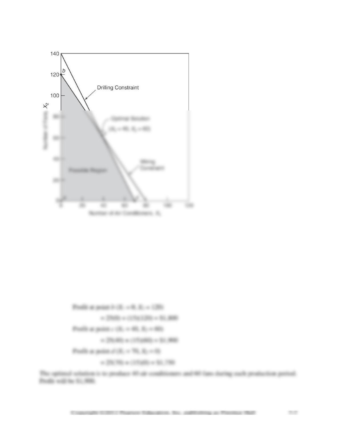
7-14.
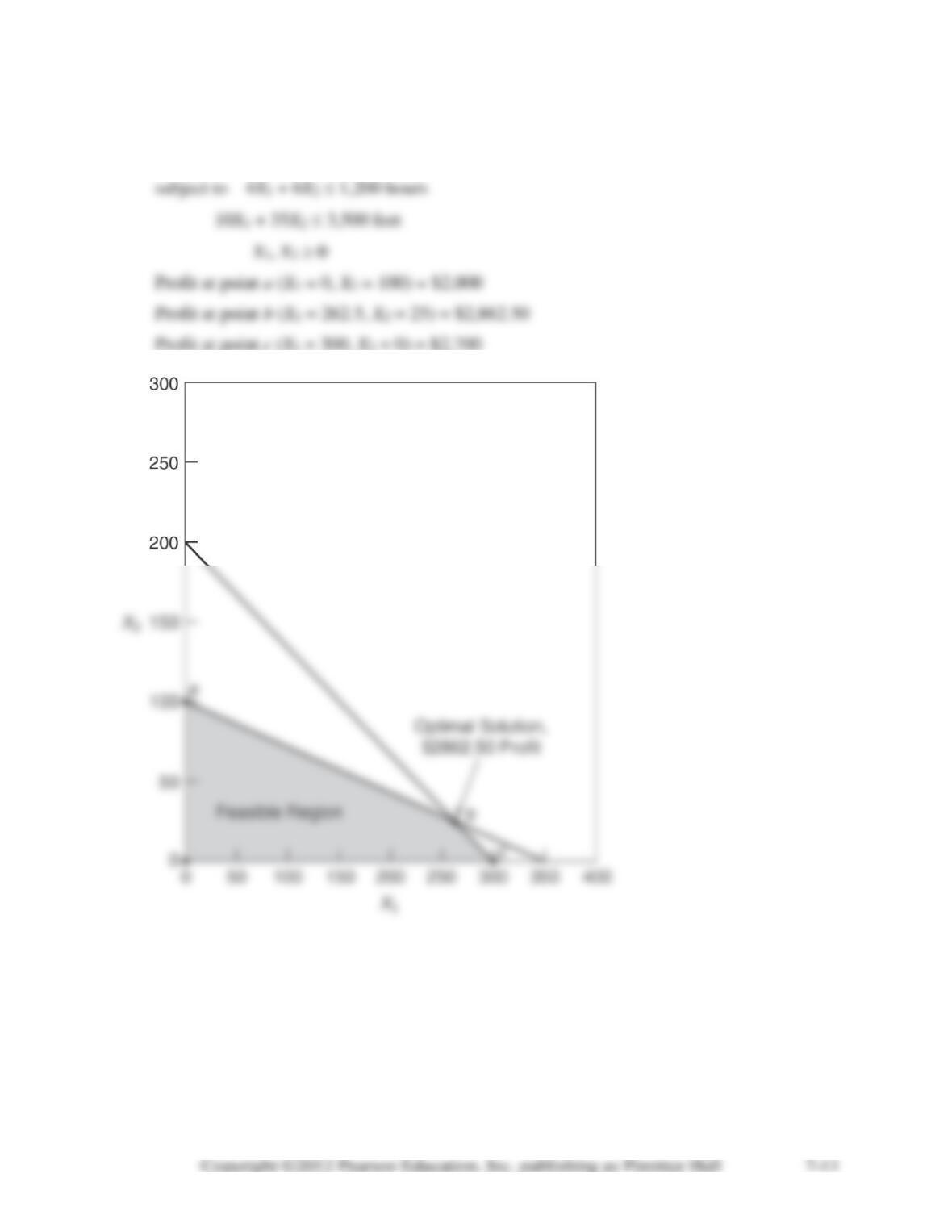
Let: X1 = number of air conditioners to be produced
X2 = number of fans to be produced
Maximize profit = 25X1 + 15X2
subject to 3X1 + 2X2 240 (wiring)
2X1 + 1X2 140 (drilling)
X1, X2 0
Profit at point a (X1 = 0, X2 = 0) = $0
7-15. a.
Maximize profit = 25X1 + 15X2
subject to 3X1 + 2X2 240
The feasible region for this problem is the combination of all of the shaded areas in Figure
7.15 above,
Profit at point a (X1 = 20, X2 = 0)
= 25(20) + (15)(0) = $500
Profit at point b (X1 = 20, X2 = 80)
= 25(20) + (15)(80) = $1,700
lution remains the same.
The calculations for the slack available at each of the four constraints at the optimal solu-
tion (40, 60) are shown below. The first two have zero slack and hence are binding constraints.
The third constraint of X1 ≥ 20 has a surplus (this is called a surplus instead of slack because the
constraint is “>“) of 20 while the fourth constraint of X2 ≤ 80 has a slack of 20.
3X1 + 2X2 + S1 = 240
so S1 = 240 – 3X1 – 2X2 = 240 – 3(40) – 2(60) = 0
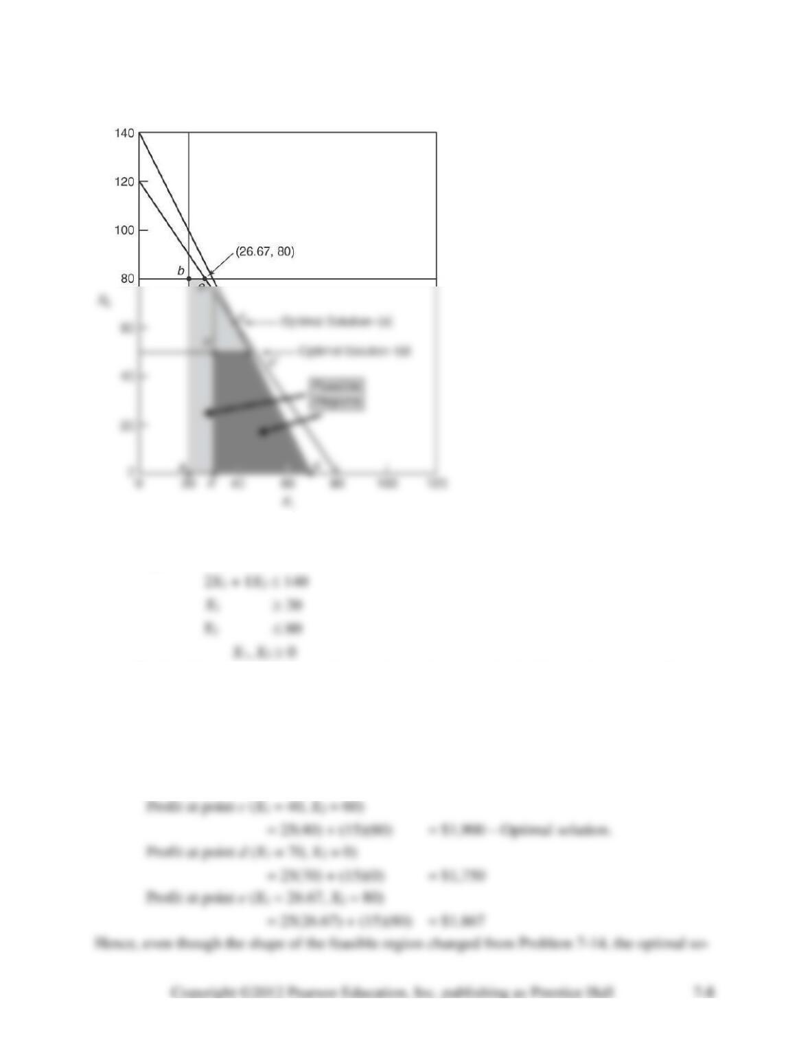
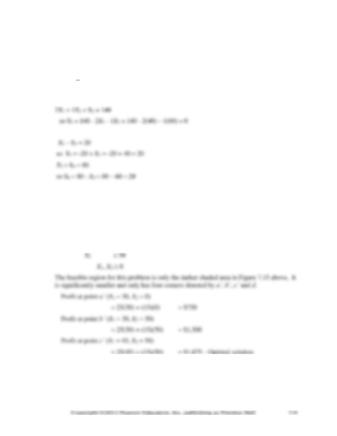
7-15. b.
Maximize profit = 25X1 + 15X2
subject to 3X1 + 2X2 240
2X1 + 1X2 140
X1 30
Profit at point d (X1 = 70, X2 = 0)
= 25(70) + (15)(0) = $1,750
Here, the shape and size of the feasible region changed and the optimal solution changed.
The calculations for the slack available at each of the four constraints at the optimal solu-
tion (45, 50) are shown below. The second and the fourth constraints have zero slack and hence
are are binding constraints. The third constraint of X1 ≥ 30 has a surplus of 15 while the first
constraint of 3X1 + 2X2 240 has a slack of 5.
7-16. Let R = number of radio ads; T = number of TV ads.
Maximize exposure = 3,000R + 7,000T
Subject to: 200R + 500T 40,000 (budget)
Optimal corner point R = 175, T = 10,
Audience = 3,000(175) + 7,000(10) = 595,000 people
7-17. X1 = number of benches produced
X2 = number of tables produced
Maximize profit = $9X1 + $20X2
7-18.
X1 = number of undergraduate courses
X2 = number of graduate courses
Minimize cost = $2,500X1 + $3,000X2
subject to X1 30
X2 20
7-19.
X1 = number of Alpha 4 computers
X2 = number of Beta 5 computers
Maximize profit = $1,200X1 + $1,800X2
subject to 20X1 + 25X2 = 800 hours
Point a is optimal.
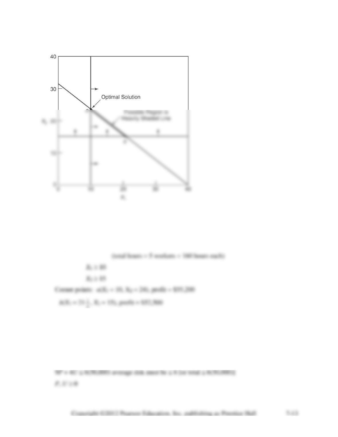
7-20. Let P = dollars invested in petrochemical; U = dollars invested in utility
Maximize return = 0.12P + 0.06U
Subject to:
P + U = 50,000 total investment is $50,000
Corner points
Return =
P
U
0.12P + 0.06U
0
50,000
3,000
30,000
4,200
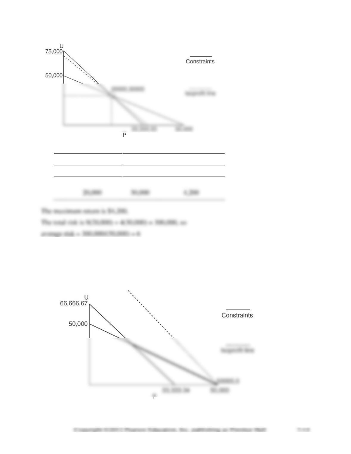
7-21. Let P = dollars invested in petrochemical; U = dollars invested in utility
Minimize risk = 9P + 4U
Subject to:
P + U = 50,000 total investment is $50,000
0.12P + 0.06U 0.08(50,000) return must be at least 8%
P, U 0
Corner points
Risk =
P
U
9P + 4U
7-22.
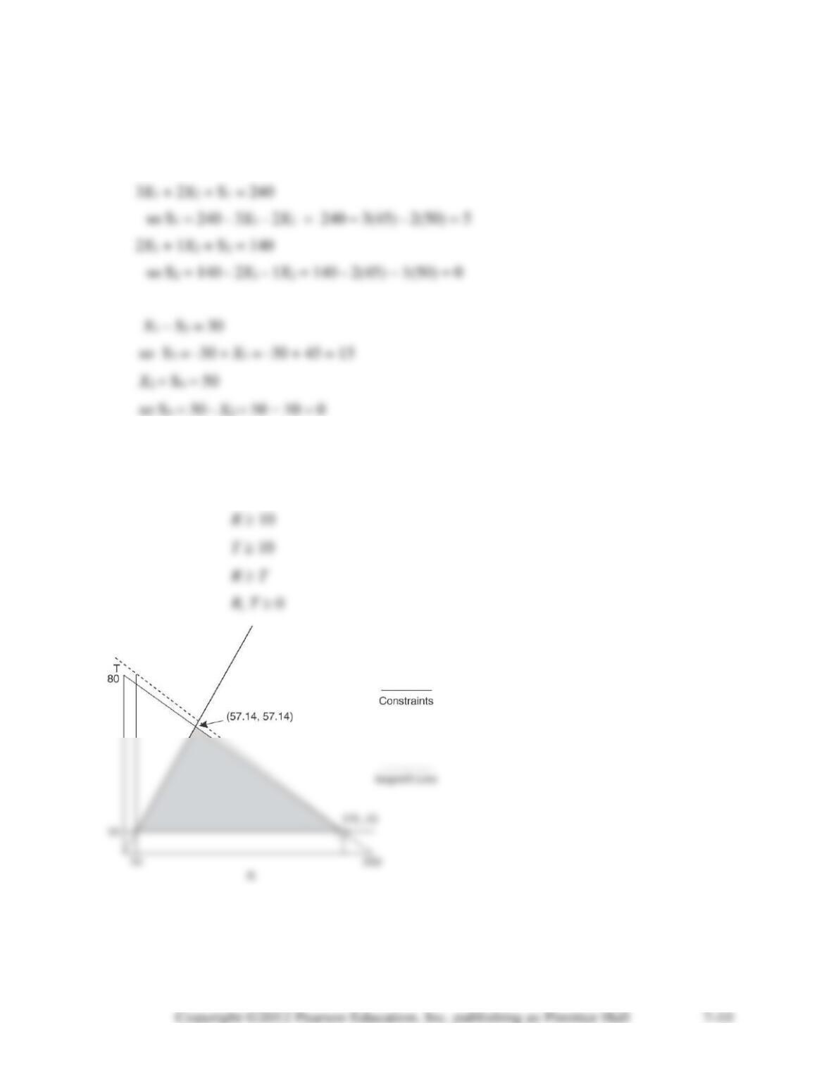
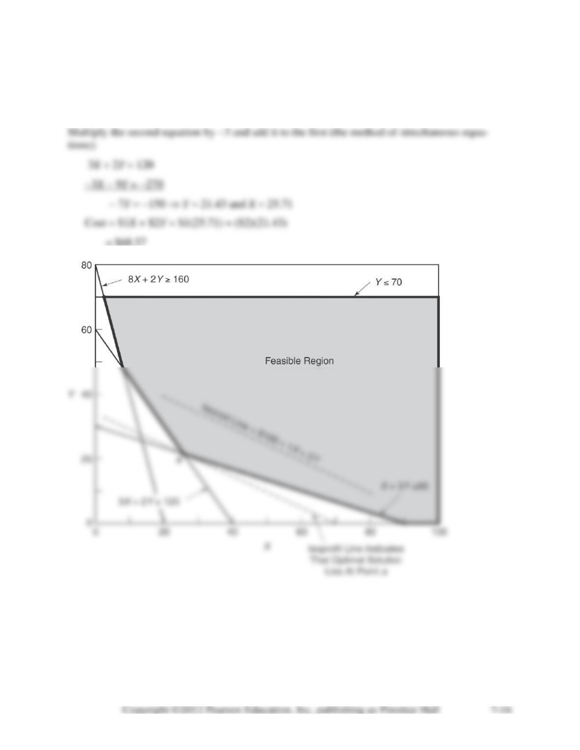
Note that this problem has one constraint with a negative sign. This may cause the beginning
student some confusion in plotting the line. As for the slack of each of the constraints, the first
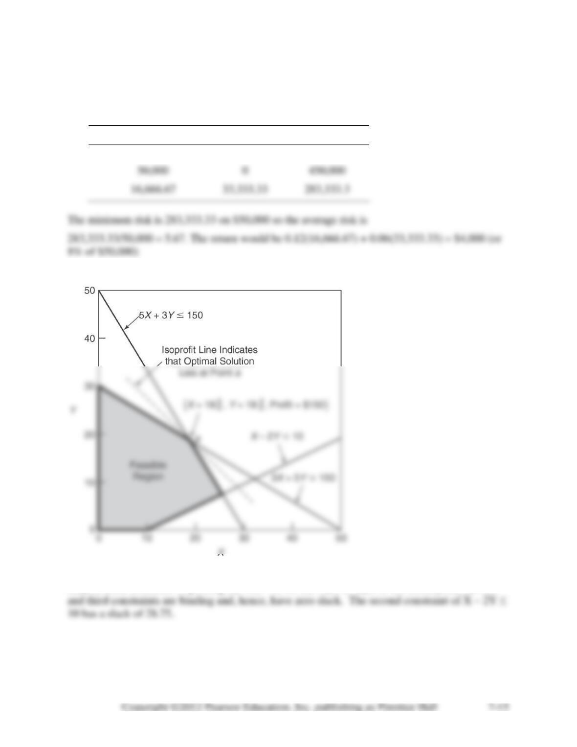
7-23. Point a lies at intersection of constraints (see figure below):
3X + 2Y = 120
X + 3Y = 90
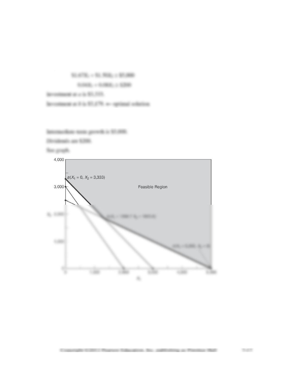
7-24. X1 = $ invested in Louisiana Gas and Power
X2 = $ invested in Trimex Insulation Co.
Minimize total investment = X1 + X2
subject to $0.36X1 + $0.24X2 $720
Investment at c is $5,000.
Short-term growth is $926.09.
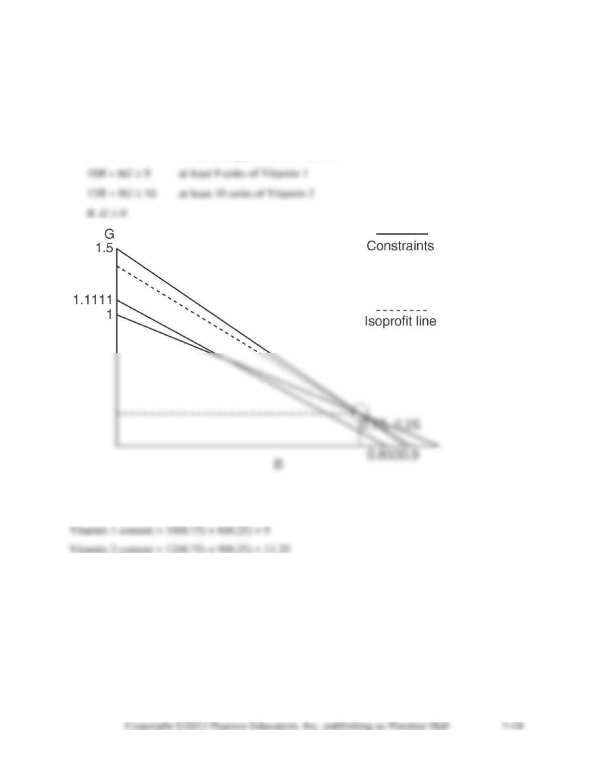
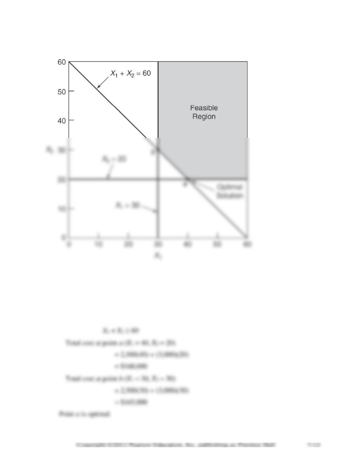
7-25. Let B = pounds of beef in each pound of dog food
G = pounds of grain in each pound of dog food
Minimize cost = 0.90B + 0.60G
Subject to:
B + G = 1 the total weight should be 1 pound
The feasible corner points are (0.75, 0.25) and (1,0). The minimum cost solution
B = 0.75 pounds of beef, G = 0.25 pounds of grain, cost = $0.825,
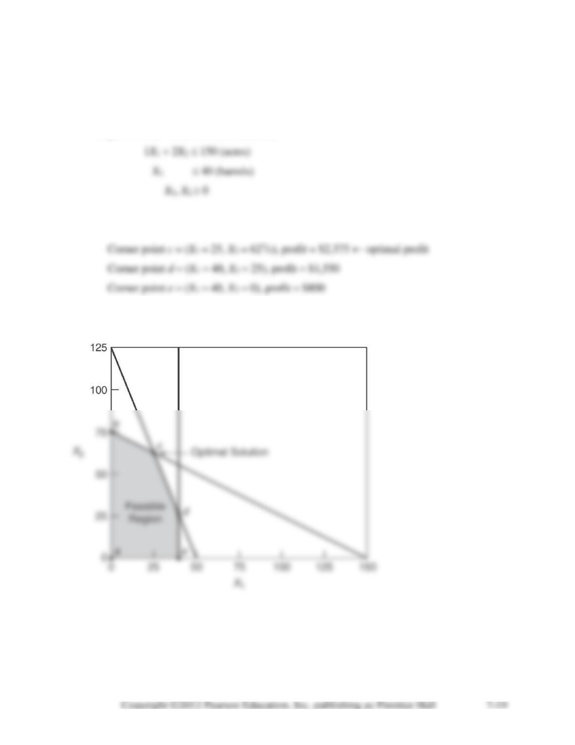
7-26. Let X1 = number of barrels of pruned olives
X2 = number of barrels of regular olives
Maximize profit = $20X1 + $30X2
subject to 5X1 + 2X2 250 (labor hours)
a. Corner point a = (X1 = 0, X2 = 0), profit = 0
Corner point b = (X1 = 0, X2 = 75), profit = $2,250
b. Produce 25 barrels of pruned olives and 621/2 barrels of regular olives.
c. Devote 25 acres to pruning process and 125 acres to regular process.
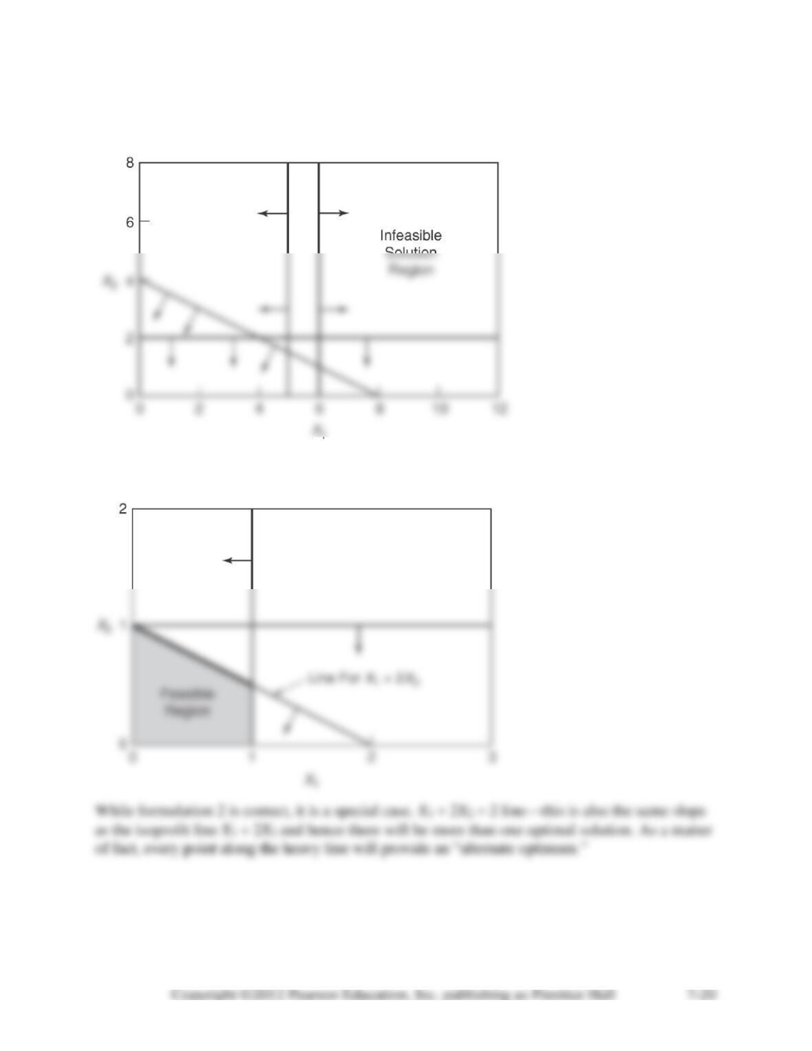
7-27.
Formulation 1:
Formulation 2: