Chapter 7
Introduction to Linear Programming
Case Problem 1: Workload Balancing
1.
Production Rate
(minutes per printer)
Model
Line 1
Line 2
Profit Contribution ($)
DI–910
3
4
42
DI–950
6
2
87
Capacity: 8 hours
60 minutes/hour = 480 minutes per day
Let D1 = number of units of the DI-910 produced
D2 = number of units of the DI-950 produced
Max
+
s.t.
The optimal solution is D1 = 0, D2 = 80. The value of the optimal solution is $6960.
Management would not implement this solution because no units of the DI-910 would be produced.
2. Adding the constraint D1 D2 and resolving the linear program results in the optimal solution D1 = 53.333,
D2 = 53.333. The value of the optimal solution is $6880.
4. Let T1 = total time spent on Line 1
T2 = total time spent on Line 2
Whatever the value of T2 is,
T1 T2 + 30
T1 T2 – 30
Chapter 7
7 – 2
Hence,
−1D1 + 4D2 30
−1D1 + 4D2 −30
Rewriting the second constraint by multiplying both sides by -1, we obtain
5. The optimal solution is D1 = 106.667, D2 = 26.667. The total profit contribution is
42(106.667) + 87(26.667) = $6800
the total time spent on each line is 480 minutes.
Case Problem 2: Production Strategy
1. `Let BP100 = the number of BodyPlus 100 machines produced
BP200 = the number of BodyPlus 200 machines produced
Max
371BP100
+
461BP200
s.t.
BP100, BP200 0
Linear Programming: Sensitivity Analysis and Interpretation of Solution
7 – 3
.
50
60
70
80
Assembly, Test, and Packaging
Machining and Welding
BP200
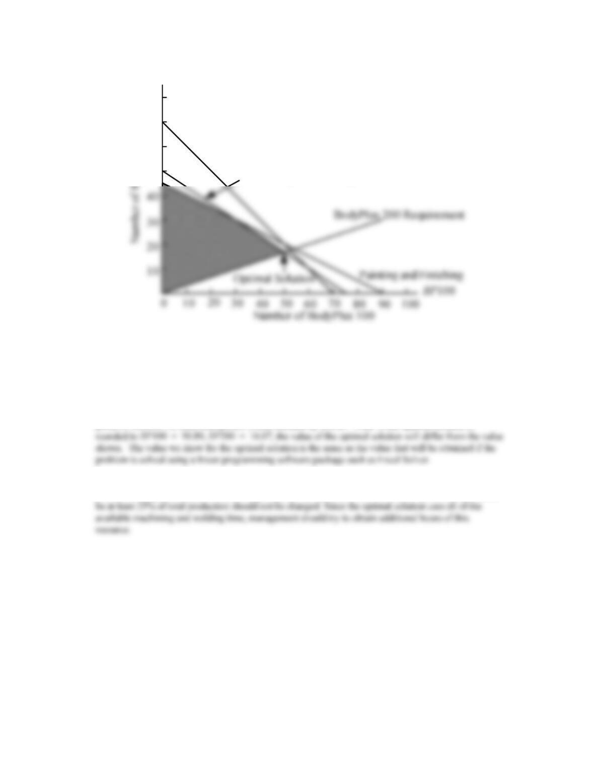
Optimal solution: BP100 = 50, BP200 = 50/3, profit = $26,233.33. Note: If the optimal solution is
rounded to BP100 = 50, BP200 = 16.67, the value of the optimal solution will differ from the value
shown. The value we show for the optimal solution is the same as the value that will be obtained if the
problem is solved using a linear programming software package such as Excel Solver.
2. In the short run the requirement reduces profits. For instance, if the requirement were reduced to at least
24% of total production, the new optimal solution is BP100 = 1425/28, BP200 = 225/14, with a total
3. If management really believes that the BodyPlus 200 can help position BFI as one of the leader’s in high-
end exercise equipment, the constraint requiring that the number of units of the BodyPlus 200 produced
Chapter 7
7 – 4
Case Problem 3: Hart Venture Capital
1. Let S = fraction of the Security Systems project funded by HVC
M = fraction of the Market Analysis project funded by HVC
Max
1,800,000S
+
1,600,000M
s.t.
600,000S
+
500,000M
600,000S
+
350,000M
700,000
Year 2
250,000S
+
400,000M
500,000
Year 3
800,000
Year 1
The answer report for this problem is shown below:
Objective Cell (Max)
Name Original Value Final Value
Net Present Value 0 2486956.522
Variable Cells
Model Variable Name Original Value Final Value Integer
Constraints
Constraint Number Name Cell Value Status Slack
1 Year 1 800000.000 Binding 0.000
Thus, the optimal solution is S = 0.609 and M = 0.870. In other words, approximately 61% of the Security
Systems project should be funded by HVC and 87% of the Market Analysis project should be funded by
HVC.
The net present value of the investment is approximately $2,486,957.
2.
Year 1
Year 2
Year 3
Security Systems
$365,217.39
$365,217.39
$152,173.91
Market Analysis
$434,782.61
$304,347.83
$347,826.09
$800,000.00
$669,565.22
3. If up to $900,000 is available in year 1 we obtain a new optimal solution with S = 0.689 and M = 0.820. In
other words, approximately 69% of the Security Systems project should be funded by HVC and 82% of the
Market Analysis project should be funded by HVC.
The net present value of the investment is approximately $2,550,820.
The answer report for this revised problem is below:
Objective Cell (Max)
Name Original Value Final Value
Variable Cells
Model Variable Name Original Value Final Value Integer
S Security Systems Project 0.000 0.689 Contin
M Market Analysis Project 0.000 0.820 Contin
Constraints
Constraint Number Name Cell Value Status Slack
1 Year 1 822950.820 Not Binding 77049.180
2 Year 2 700000.000 Binding 0.000
4. If an additional $100,000 is made available, the allocation plan would change as follows (again, using non-
rounded values for S and M):
Year 1
Year 2
Year 3
Security Systems
$413,114.75
$413,114.750
$172,250
Market Analysis
$409,836.07
$286,885.25
$328,000
Total
$822,950.82
$700,000.00
$500,000.00
5. Having additional funds available in year 1 will increase the total net present value. The value of the objective
function increases from $2,486,957 to $2,550,820, a difference of $63,863. But, since the allocation plan
shows that $822,951 is required in year 1, only $22,951 of the additional $100,00 is required. We can also