Chapter 17
The data appear to follow a horizontal pattern.
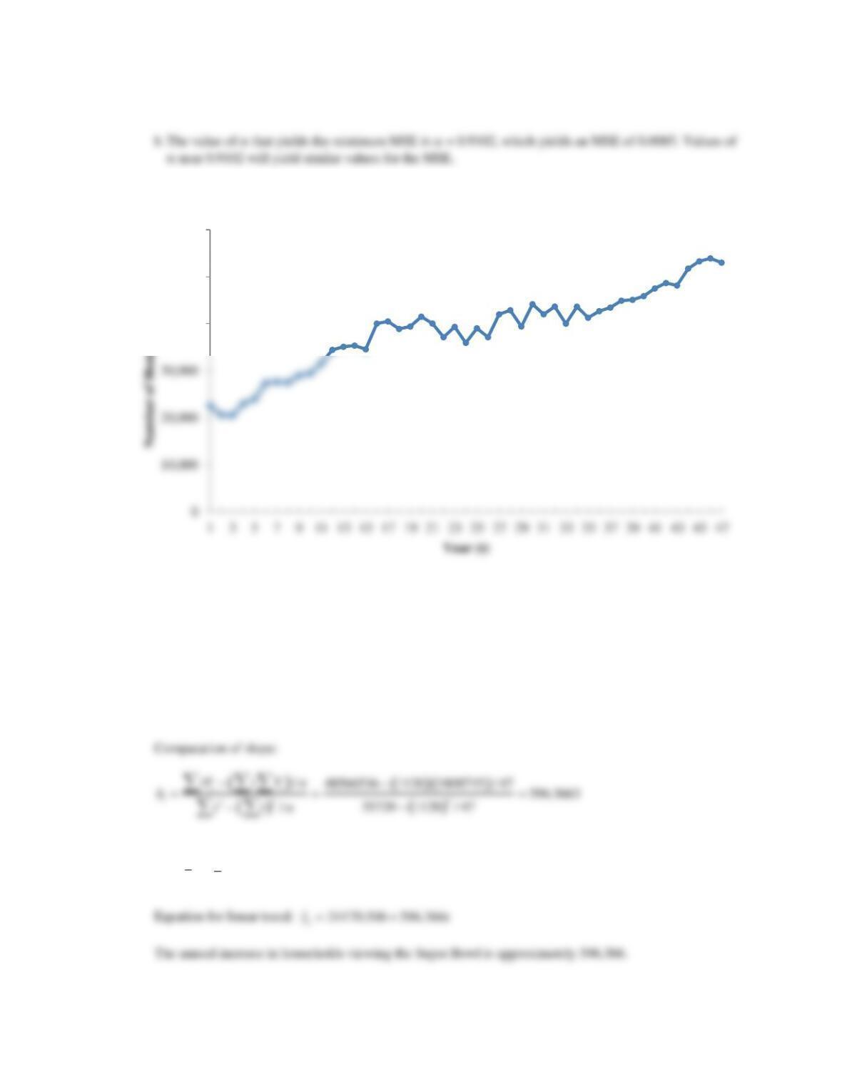
16. a.
b. This time series plot indicates a possible linear trend in the data, so forecasting methods discussed in
this chapter are appropriate to develop forecasts for this time series.
c. The following values are needed to compute the slope and intercept:
2
1128 35720 1808715 48566536
tt
t t Y tY= = = =
Computation of intercept:
01
b Y b t= − =
(38483.30/47) – (596.366)(1128/47) = 24170.506
40,000
50,000
60,000
Markov Processes
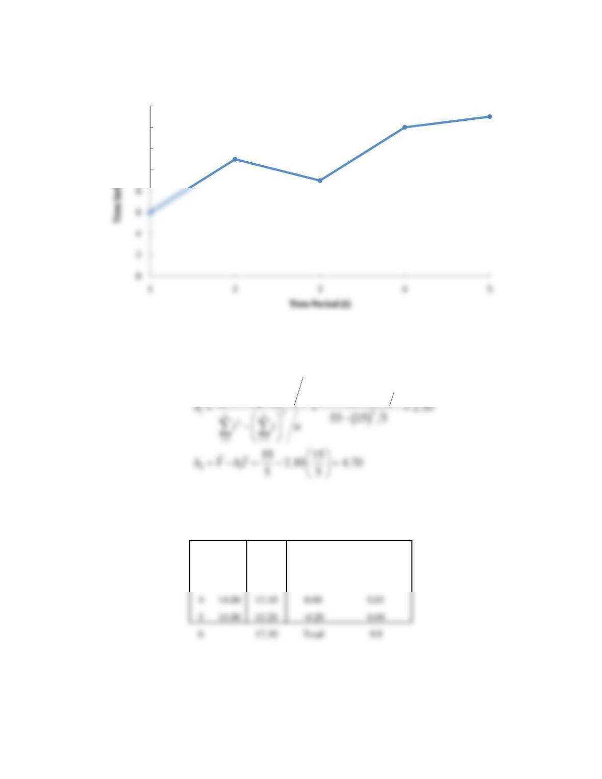
17. a.
The time series plot shows a linear trend.
b. The regression estimates for the slope and y-intercept are
( )( )
186 15 55 5 2.10
n n n
tt
tY t Y n
−−
which results in the following forecasts, errors, and MSE:
Year
Sales
Forecast
Forecast
Error
Squared
Forecast Error
1
6.00
6.80
-0.80
0.64
2
11.00
8.90
2.10
4.41
3
9.00
11.00
-2.00
4.00
4
14.00
13.10
0.90
0.81
5
15.00
15.20
-0.20
0.04
6
17.30
Total
MSE = 9.9/5 = 1.982.475.
c.
6
ˆ
y
= b0 + b1t = 4.7 + 2.1(6) = 17.3
10
12
14
16
Chapter 17
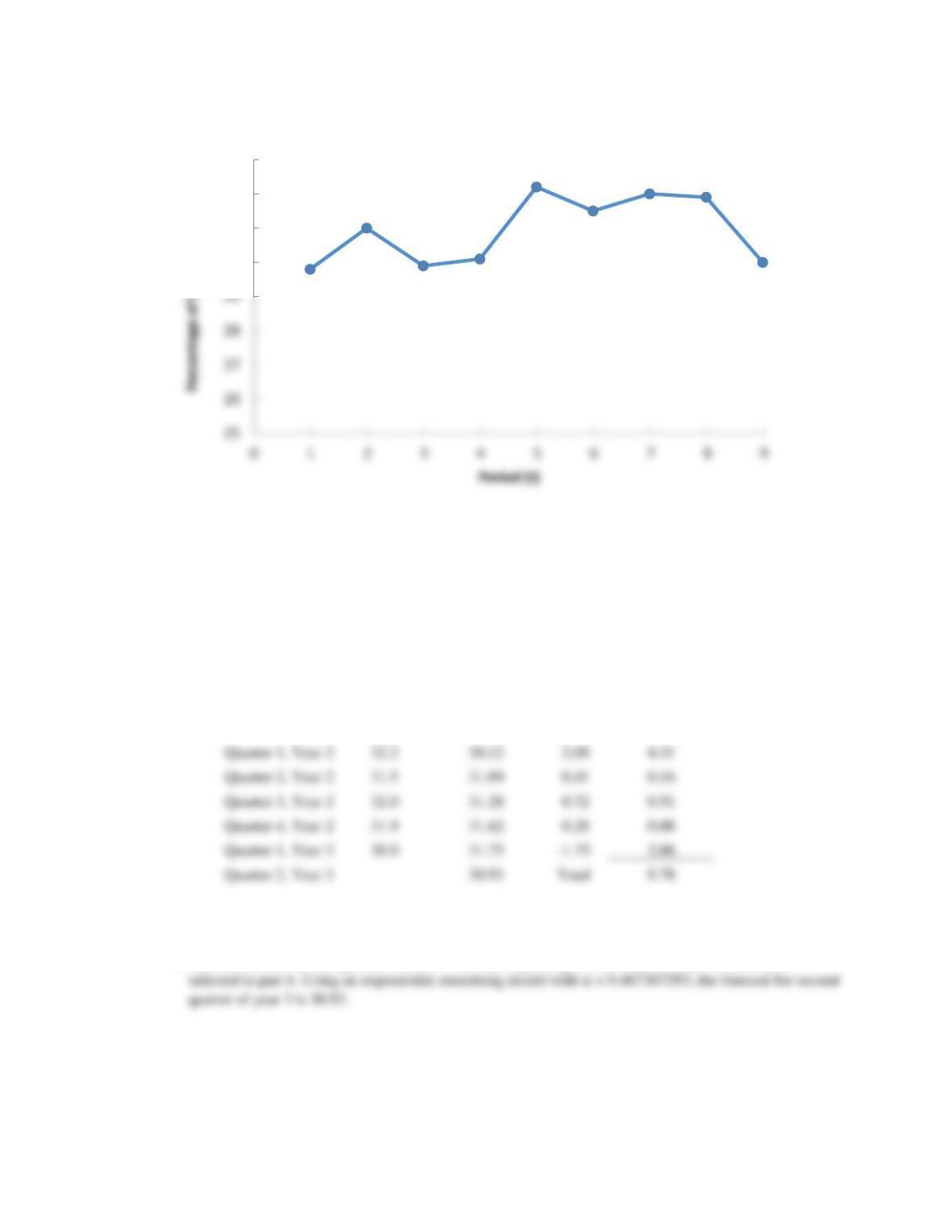
18. a.
b. The value of the MSE will vary depending on the ultimate value of that you select. The value of
that yields the smallest possible MSE is = 0.467307293, which yields an MSE of 1.222838367.
Alpha
0.467307293
Period
Stock %
Forecast
Forecast
Error
Squared
Forecast Error
Quarter 1, Year 1
29.8
Quarter 2, Year 1
31.0
29.80
1.20
1.44
Quarter 3, Year 1
29.9
30.36
-0.46
0.21
Quarter 4, Year 1
30.1
30.15
-0.05
0.00
Quarter 1, Year 2
32.2
30.12
2.08
4.31
Quarter 2, Year 2
31.5
31.09
0.41
0.16
Quarter 3, Year 2
32.0
31.28
0.72
0.51
Quarter 4, Year 2
31.9
31.62
0.28
0.08
Quarter 1, Year 3
30.0
31.75
-1.75
3.06
Quarter 2, Year 3
30.93
Total
9.78
MSE =
1.222838367
c. The forecast for second quarter of year 3 will vary depending on the ultimate value of that you
30
31
32
33
Markov Processes
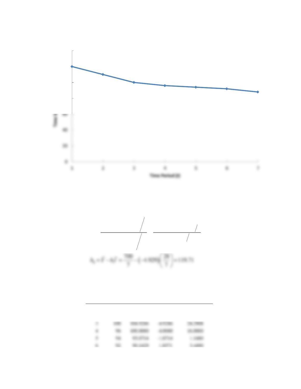
19. a.
The data are following a downward trend.
b. The regression estimates for the slope and y-intercept for the line that minimizes MSE for this time
series are
( )( )
( )
1 1 1
122
2
11
2662 28 700 7 4.929
140 28 7
n n n
tt
t t t
nn
tt
tY t Y n
b
t t n
= = =
==
−−
= = = −
−
−
which results in the following forecasts, errors, and MSE:
Period
Time
Series
Value
Forecast
Forecast
Error
Squared
Forecast
Error
1
120
114.7857
5.2143
27.1888
2
110
109.8571
0.1429
0.0204
3
100
104.9286
24.2908
4
100.0000
16.0000
80
100
120
140
Chapter 17
7
88
85.2143
2.7857
7.7602
Total
79.8571
MSE = 79.8571 / 7 = 11.408.
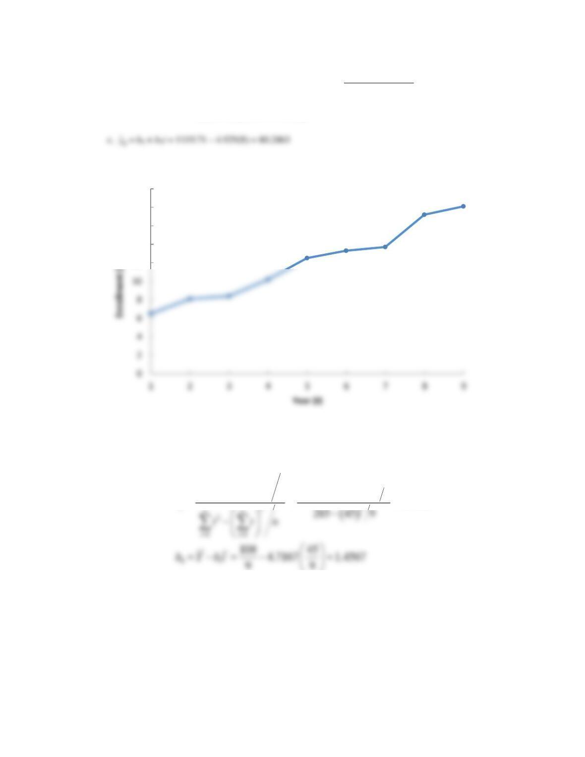
20. a.
The time series plot shows a linear trend
b. The regression estimates for the slope and y-intercept are
( )( )
1 1 1
627.4 45 108 9 4.7167
n n n
tt
t t t
tY t Y n
b
= = =
−−
= = =
12
14
16
18
20
Markov Processes
which results in the following forecasts, errors, and MSE:
Period
Year
Enrollment
Forecast
Forecast
Error
Squared
Forecast
Error
1
2001
6.50
6.17
0.33
0.11
2
2002
8.10
7.63
0.47
0.22
3
2003
8.40
9.09
-0.69
0.47
4
2004
10.20
10.54
-0.34
0.12
5
2005
12.50
12.00
0.50
0.25
6
2006
13.30
13.46
-0.16
0.02
7
2007
13.70
14.91
-1.21
1.47
8
2008
17.20
16.37
0.83
0.69
9
2009
18.10
17.83
0.27
0.07
2010
19.28
MSE =
0.3808148
c.
10
ˆ
y
= b0 + b1t = 4.7167 + 1.4567(10) = 19.28
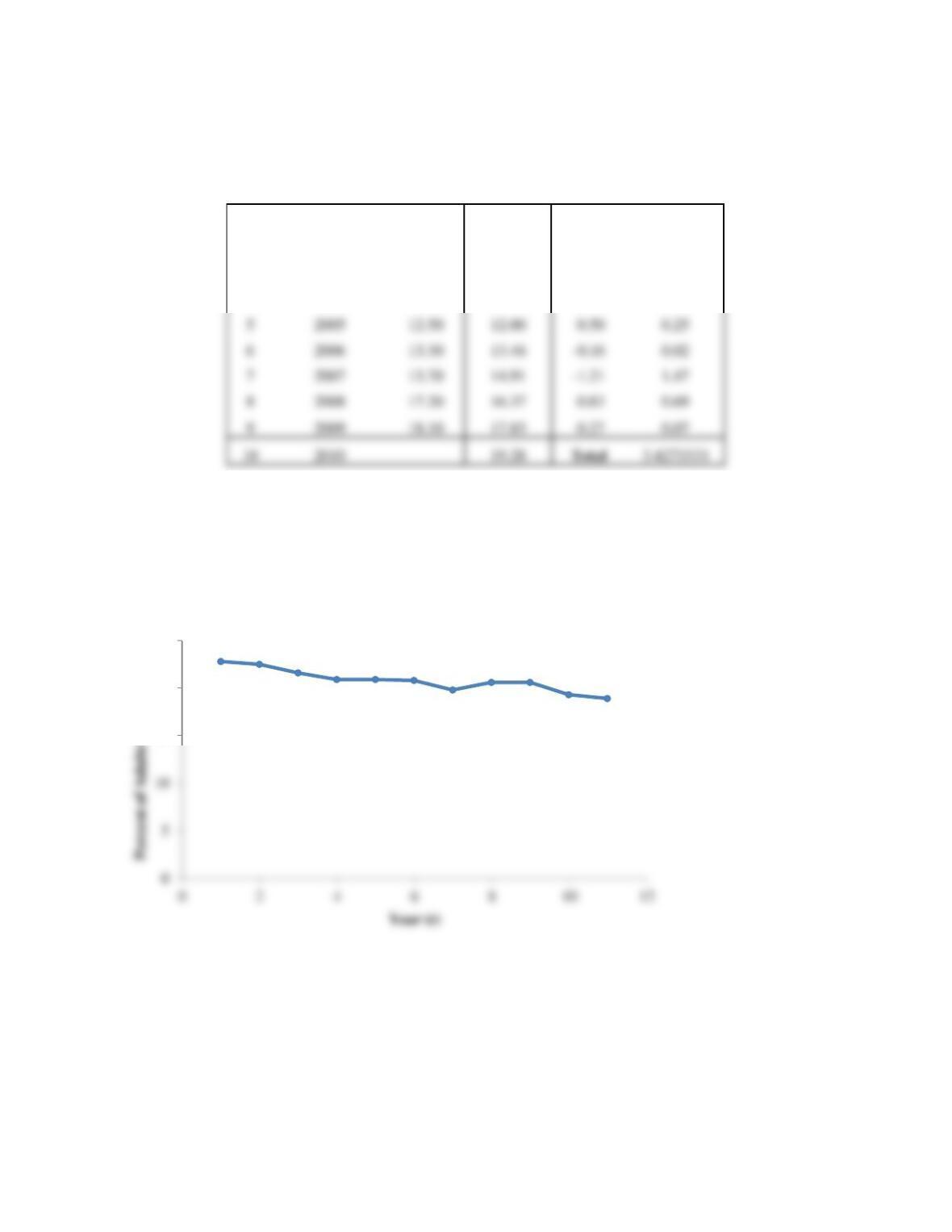
21. a.
This time series plot indicates a possible negative linear trend in the data.
b. The following values are needed to compute the slope and intercept:
2
66 506 228.7 1335.2
tt
t t Y tY= = = =
15
20
25
Chapter 17
Computation of slope:
( )
( )
( )( )
( )
122
2
/1335.2 66 228.7 /11 0.3364
506 66 /11
/
tt
tY t Y n
b
t t n
−−
= = =
−
−
c. The forecast of the percent of adults who smoke nine years after these data have been collected is
( )
20
ˆ22.89096 0.3364 20 16.0818y= − =
. The regression model from part (b) does suggest that the OSH is
not on target to meet this goal.
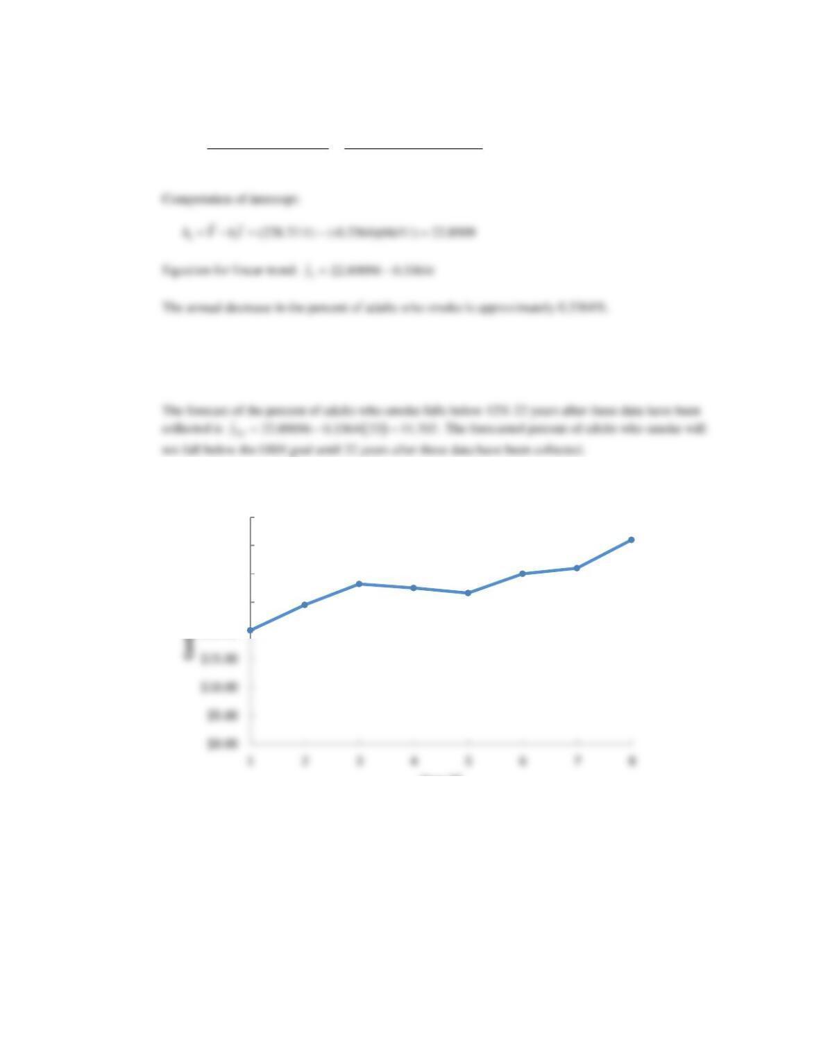
22. a.
The time series plot shows an upward linear trend
$20.00
$25.00
$30.00
$35.00
$40.00
Year (t)
Markov Processes
b. The regression estimates for the slope and y-intercept are
( )( )
( )
1 1 1
122
2
11
1081.6 36 223.8 8 1.7738
204 36 8
n n n
tt
t t t
nn
tt
tY t Y n
b
t t n
= = =
==
−−
= = =
−
−
Squared
Forecast
Forecast
Year
Cost/Unit($)
Forecast
Error
Error
1
20.00
21.77
-1.77
3.12
2
24.50
23.54
0.96
0.92
3
28.20
25.31
2.89
8.33
4
27.50
27.09
0.41
0.17
5
26.60
28.86
-2.26
5.12
6
30.00
30.64
-0.64
0.40
7
31.00
32.41
-1.41
1.99
8
36.00
34.18
1.82
3.30
Total
23.34619
MSE =
2.9183
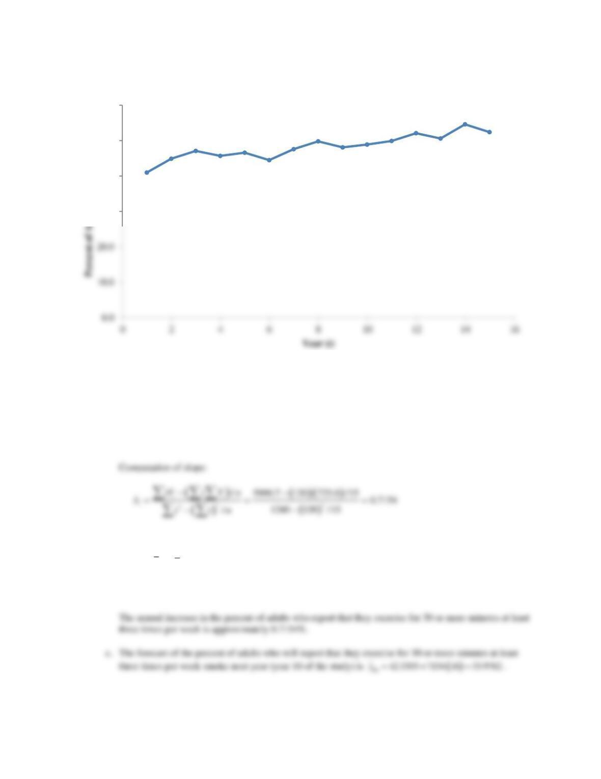
c. The average cost/unit has been increasing by approximately $1.77 per year.
Chapter 17
23. a.
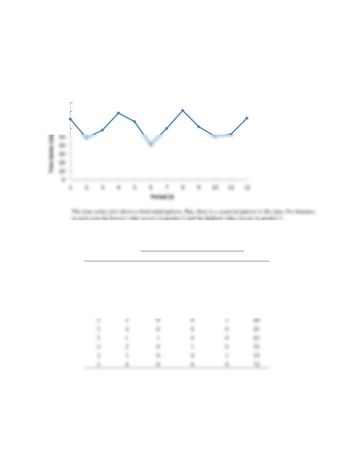
This time series plot indicates a possible positive linear trend in the data.
b. The following values are needed to compute the slope and intercept:
2
120 1240 723.8 5990.7
tt
t t Y tY= = = =
Computation of intercept:
01
b Y b t= − =
(723.8/15) – (0.7154)(120/15) = 42.5305
Equation for linear trend:
ˆ42.5305 0.7154
t
yt
=+
30.0
40.0
50.0
60.0
Markov Processes
d. The linear trend we observed in the time series plot from part (a) appears to be stable, so the trend
equation from part (b) can be used to forecast the percentage of adults three years from now (year 18 of
the study) who will report that they exercise for 30 or more minutes at least three times per week. The
forecast of the percent of adults who will report that they exercise for 30 or more minutes at least three
times per week smoke three years from now (year 18 of the study) is
( )
18
ˆ42.5305 7154 18 55.4069y= + =
24. a.
b. After putting the data into the following format:
Dummy Variables
Year
Quarter
Quarter 1
Quarter 2
Quarter 3
Yt
1
1
1
0
0
71
1
2
0
1
0
48
1
3
0
0
1
58
1
4
0
0
0
78
2
1
1
0
0
68
2
2
0
1
0
41
2
3
0
0
1
60
2
4
0
0
0
81
3
1
1
0
0
62
3
2
0
1
0
51
3
3
0
0
1
53
3
4
0
0
0
72
we can use the LINEST function to find the regression model:
Value = 77.00 – 10.00 Qtr1 – 30.33 Qtr2 – 20.00 Qtr3
c. The quarterly forecasts for next year are as follows:
60
70
80
90
Chapter 17
Quarter 1 forecast = 77.0 – 10.0(1) – 30.33(0) – 20.0(0) = 67.00
Quarter 2 forecast = 77.0 – 10.0(0) – 30.33(1) – 20.0(0) = 46.67
25. a.
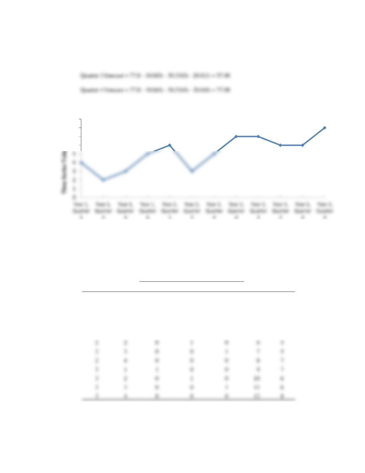
Careful scrutiny of the time series plot reveals a horizontal pattern with a seasonality. For instance, in
each year the value drops from quarter 1 to quarter 2 and the value increases from quarter 3 to quarter 4.
b. After putting the data into the following format:
Dummy Variables
Year
Quarter
Quarter 1
Quarter 2
Quarter 3
T
Yt
1
1
1
0
0
1
4
1
2
0
1
0
2
2
1
3
0
0
1
3
3
1
4
0
0
0
4
5
2
1
1
0
0
5
6
2
2
0
1
0
6
3
2
3
0
0
1
7
5
2
4
0
0
0
8
7
3
1
1
0
0
9
7
3
2
0
1
0
6
3
3
0
0
1
6
3
4
0
0
0
8
we develop the following estimated regression coefficients to account for trend and seasonal effects in
the data by using the LINEST function:
6
7
8
9
Time Period
Markov Processes
b0 = 3.417 b1 = 0.219 b2 = -2.188 b3 = -1.594 bt = 0.406
Thus, the linear regression that accounts for trend and seasonal effects in the data is:
Value = 3.417 + 0.219 Qtr1 – 2.188 Qtr2 – 1.594 Qtr3 + 0.406 t
c. The quarterly forecasts for next year are as follows:
Quarter 1 forecast = 3.417 + 0.219(1) – 2.188(0) – 1.594(0) + 0.406(13) = 8.92
26. a.
2000
2500
3000
3500
Chapter 17
b. After putting the data into the following format:
Dummy Variables
Year
Quarter
Quarter 1
Quarter 2
Quarter 3
Yt
1
1
1
0
0
1690
1
2
0
1
0
940
1
3
0
0
1
2625
1
4
0
0
0
2500
2
1
1
0
0
1800
2
2
0
1
0
900
2
3
0
0
1
2900
2
4
0
0
0
2360
3
1
1
0
0
1850
3
2
0
1
0
1100
3
3
0
0
1
2930
3
4
0
0
0
2615
c. The quarterly forecasts for next year are as follows:
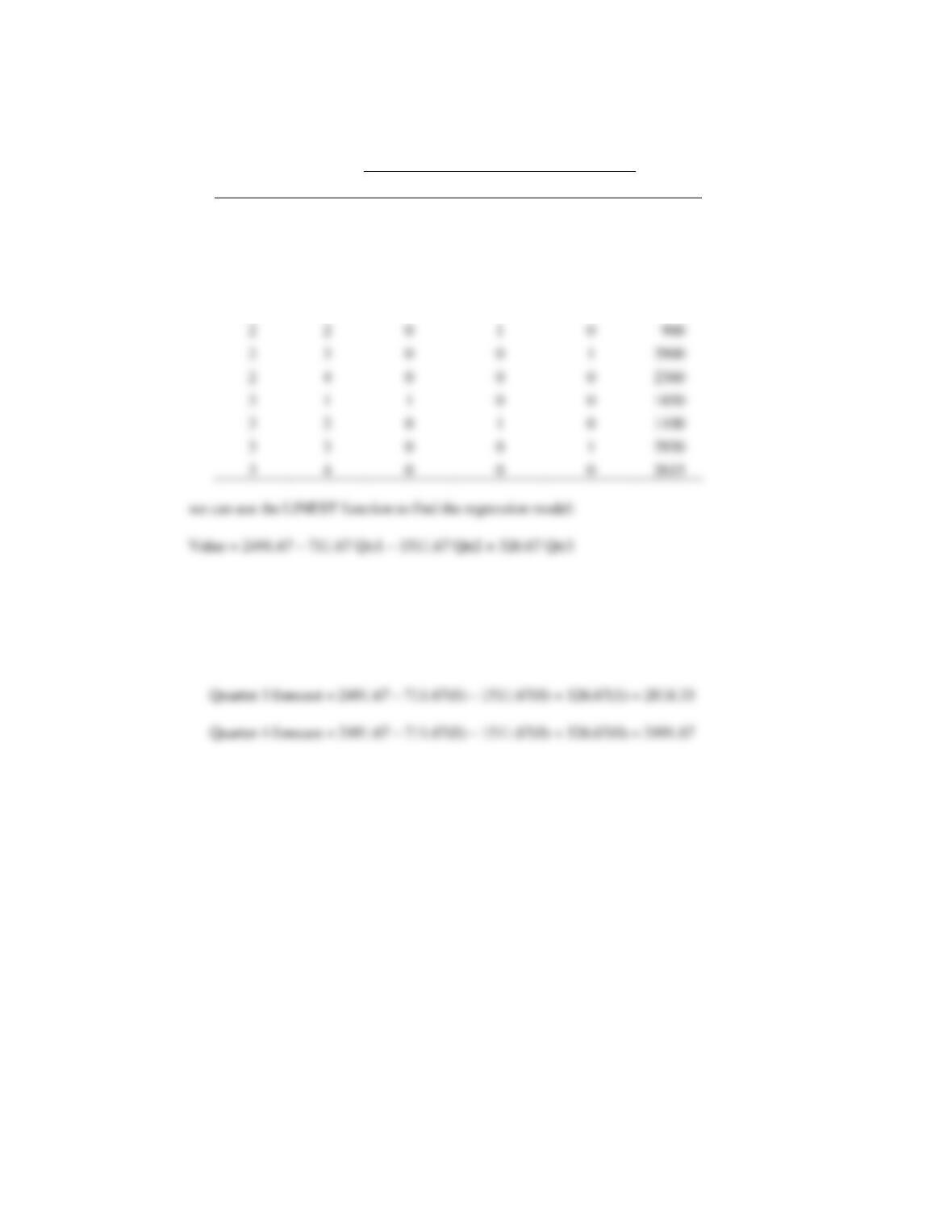
Quarter 1 forecast = 2491.67 – 711.67(1) – 1511.67(0) + 326.67(0) = 1780.00
Quarter 2 forecast = 2491.67 – 711.67(0) – 1511.67(1) + 326.67(0) = 980.00
Markov Processes
d. After putting the data into the following format:
Dummy Variables
Year
Quarter
Quarter 1
Quarter 2
Quarter 3
t
Yt
1
1
1
0
0
1
1690
1
2
0
1
0
2
940
1
3
0
0
1
3
2625
1
4
0
0
0
4
2500
2
1
1
0
0
5
1800
2
2
0
1
0
6
900
2
3
0
0
1
7
2900
2
4
0
0
0
8
2360
3
1
1
0
0
9
1850
3
2
0
1
0
1100
3
3
0
0
1
2930
3
4
0
0
0
2615
we can use the LINEST function to find the regression model:
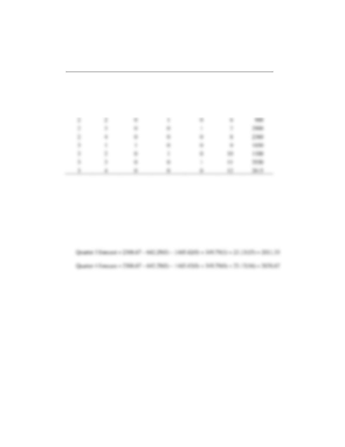
Value = 2306.67 – 642.29 Qtr1 – 1465.42 Qtr2 + 349.79 Qtr3 + 23.13t
The quarterly forecasts for next year are as follows:
Quarter 1 forecast = 2306.67 – 642.29(1) – 1465.42(0) + 349.79(0) + 23.13(13) = 1965.00
Quarter 2 forecast = 2306.67 – 642.29(0) – 1465.42(1) + 349.79(0) + 23.13(14) = 1165.00
27. a.
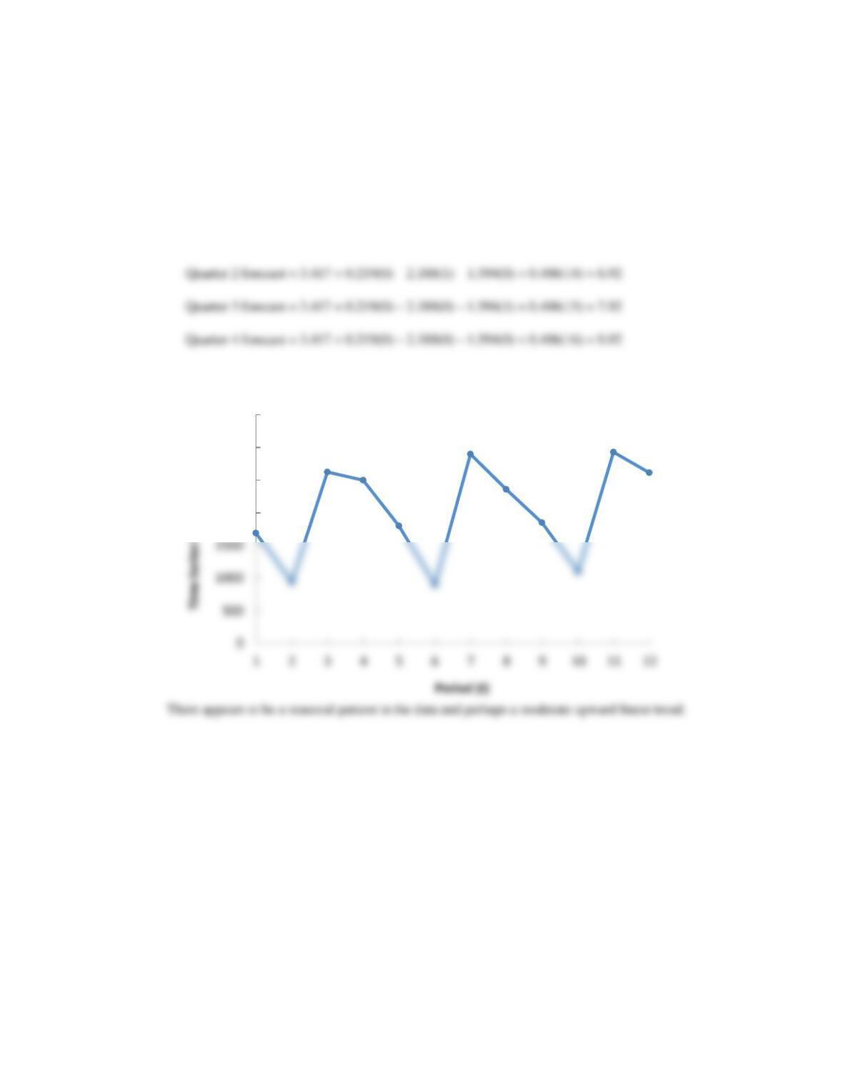
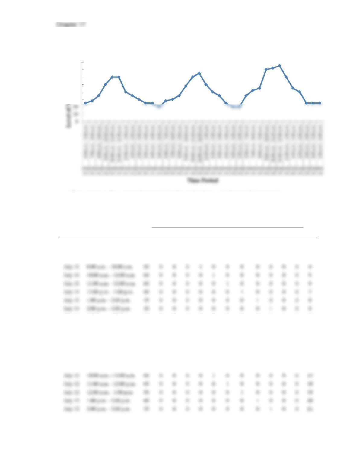
There appears to be a seasonal pattern in the data and perhaps a slight upward linear trend.
b. After putting the data into the following format:
Hourly Dummy Variables
Date
Hour
Yt
1
2
3
4
5
6
7
8
9
10
11
t
July 11
6:00 a.m. – 7:00 a.m.
25
1
0
0
0
0
0
0
0
0
0
0
1
July 11
7:00 a.m. – 8:00 a.m.
28
0
1
0
0
0
0
0
0
0
0
0
2
July 11
8:00 a.m. – 9:00 a.m.
35
0
0
1
0
0
0
0
0
0
0
0
3
July 11
9:00 a.m. – 10:00 a.m.
50
0
0
0
1
0
0
0
0
0
0
0
4
July 11
10:00 a.m. – 11:00 a.m.
60
0
0
0
0
1
0
0
0
0
0
0
5
July 11
11:00 a.m. – 12:00 p.m.
60
0
0
0
0
0
1
0
0
0
0
0
6
July 11
12:00 p.m. – 1:00 p.m.
40
0
0
0
0
0
0
1
0
0
0
0
7
July 11
1:00 p.m. – 2:00 p.m.
35
0
0
0
0
0
0
0
1
0
0
0
8
July 11
2:00 p.m. – 3:00 p.m.
30
0
0
0
0
0
0
0
0
1
0
0
9
July 11
3:00 p.m. – 4:00 p.m.
25
0
0
0
0
0
0
0
0
0
1
0
10
July 11
4:00 p.m. – 5:00 p.m.
25
0
0
0
0
0
0
0
0
0
0
1
11
July 11
5:00 p.m. – 6:00 p.m.
20
0
0
0
0
0
0
0
0
0
0
0
12
July 12
6:00 a.m. – 7:00 a.m.
28
1
0
0
0
0
0
0
0
0
0
0
13
July 12
7:00 a.m. – 8:00 a.m.
30
0
1
0
0
0
0
0
0
0
0
0
14
July 12
8:00 a.m. – 9:00 a.m.
35
0
0
1
0
0
0
0
0
0
0
0
15
July 12
9:00 a.m. – 10:00 a.m.
48
0
0
0
1
0
0
0
0
0
0
0
16
July 12
10:00 a.m. – 11:00 a.m.
60
0
0
0
0
1
0
0
0
0
0
0
17
July 12
11:00 a.m. – 12:00 p.m.
65
0
0
0
0
0
1
0
0
0
0
0
18
July 12
12:00 p.m. – 1:00 p.m.
50
0
0
0
0
0
0
1
0
0
0
0
19
30
40
50
60
70
80
Markov Processes
July 12
3:00 p.m. – 4:00 p.m.
25
0
0
0
0
0
0
0
0
0
1
0
22
July 12
4:00 p.m. – 5:00 p.m.
20
0
0
0
0
0
0
0
0
0
0
1
23
July 12
5:00 p.m. – 6:00 p.m.
20
0
0
0
0
0
0
0
0
0
0
0
24
July 13
6:00 a.m. – 7:00 a.m.
35
1
0
0
0
0
0
0
0
0
0
0
25
July 13
7:00 a.m. – 8:00 a.m.
42
0
1
0
0
0
0
0
0
0
0
0
26
July 13
8:00 a.m. – 9:00 a.m.
45
0
0
1
0
0
0
0
0
0
0
0
27
July 13
9:00 a.m. – 10:00 a.m.
70
0
0
0
1
0
0
0
0
0
0
0
28
July 13
10:00 a.m. – 11:00 a.m.
72
0
0
0
0
1
0
0
0
0
0
0
29
July 13
11:00 a.m. – 12:00 p.m.
75
0
0
0
0
0
1
0
0
0
0
0
30
July 13
12:00 p.m. – 1:00 p.m.
60
0
0
0
0
0
0
1
0
0
0
0
31
July 13
1:00 p.m. – 2:00 p.m.
45
0
0
0
0
0
0
0
1
0
0
0
32
July 13
2:00 p.m. – 3:00 p.m.
40
0
0
0
0
0
0
0
0
1
0
0
33
July 13
3:00 p.m. – 4:00 p.m.
25
0
0
0
0
0
0
0
0
0
1
0
34
July 13
4:00 p.m. – 5:00 p.m.
25
0
0
0
0
0
0
0
0
0
0
1
35
July 13
5:00 p.m. – 6:00 p.m.
25
0
0
0
0
0
0
0
0
0
0
0
36
we develop the following estimated regression coefficients to account for trend and seasonal effects in
the data by using the LINEST function:
b0 =
11.167
b1 =
12.479
b2 =
16.042
b3 =
20.604
b4 =
37.833
b5 =
45.396
b6 =
47.625
b7 =
30.521
b8 =
20.083
b9 =
14.646
Thus, the linear regression that accounts for trend and seasonal effects in the data is:
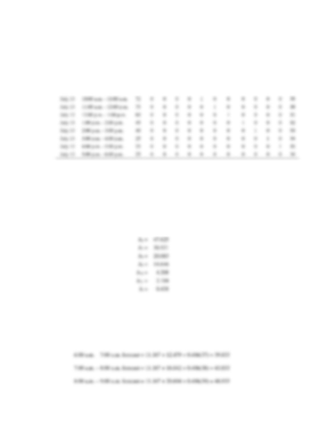
Value = 11.167 + 12.479HOUR2 + 16.042HOUR3 + 20.604HOUR4 + 37.833HOUR5 +
45.396HOUR6 + 47.625HOUR7 + 30.521HOUR8 + 20.083HOUR9 + 14.646HOUR10 +
4.208HOUR11 + 2.104HOUR12 + 0.438t
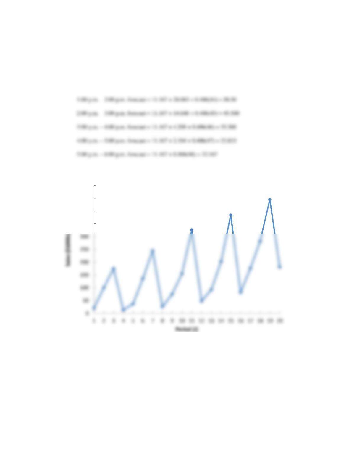
c. The hourly forecasts for July 14 (t = 37 through t = 48) are as follows:
Chapter 17
9:00 a.m. – 10:00 a.m. forecast = 11.167 + 37.833 + 0.406(40) = 66.500
10:00 a.m. – 11:00 a.m. forecast = 11.167 + 45.396 + 0.406(41) = 74.500
11:00 a.m. – noon forecast = 11.167 + 47.625 + 0.406(42) = 77.167
noon – 1:00 p.m. forecast = 11.167 + 30.521 + 0.406(43) = 60.50
28. a.
The time series plot shows both a linear trend and seasonal effects.
350
400
450
500
Markov Processes
b. After putting the data into the following format:
Dummy Variables
Year
Quarter
Quarter 1
Quarter 2
Quarter 3
Yt
1
1
1
0
0
20
1
2
0
1
0
100
1
3
0
0
1
175
1
4
0
0
0
13
2
1
1
0
0
37
2
2
0
1
0
136
2
3
0
0
1
245
2
4
0
0
0
26
3
1
1
0
0
75
3
2
0
1
0
155
3
3
0
0
1
326
3
4
0
0
0
48
4
1
1
0
0
92
4
2
0
1
0
202
4
3
0
0
1
384
4
4
0
0
0
82
5
1
1
0
0
176
5
2
0
1
0
282
5
3
0
0
1
445
5
4
0
0
0
181
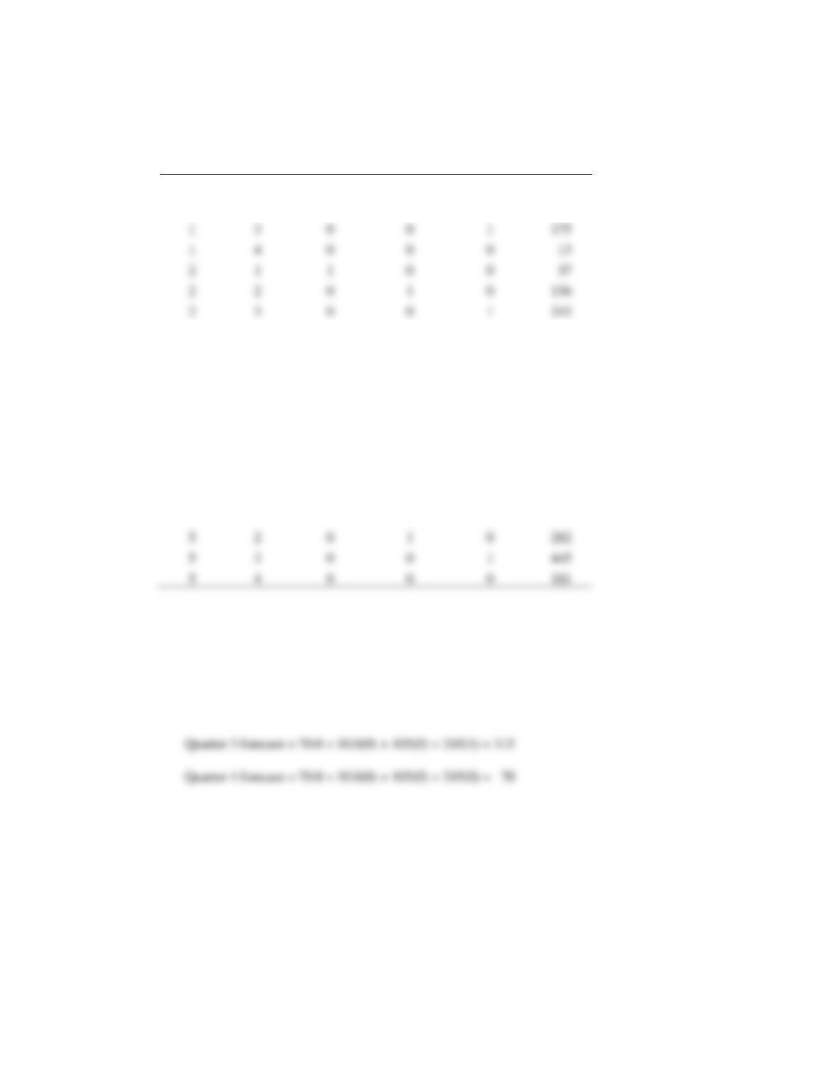
we can use the LINEST function to find the regression model:
Revenue = 70.0 + 10.0 Qtr1 + 105 Qtr2 + 245 Qtr3
Quarter 1 forecast = 70.0 + 10.0(1) + 105(0) + 245(0) = 80
Quarter 2 forecast = 70.0 + 10.0(0) + 105(1) + 245(0) = 175
Chapter 17
c. After putting the data into the following format:
Dummy Variables
Year
Quarter
Quarter 1
Quarter 2
Quarter 3
t
Yt
1
1
1
0
0
1
20
1
2
0
1
0
2
100
1
3
0
0
1
3
175
1
4
0
0
0
4
13
2
1
1
0
0
5
37
2
2
0
1
0
6
136
2
3
0
0
1
7
245
2
4
0
0
0
8
26
3
1
1
0
0
9
75
3
2
0
1
0
10
155
3
3
0
0
1
11
326
3
4
0
0
0
12
48
4
1
1
0
0
13
92
4
2
0
1
0
14
202
4
3
0
0
1
15
384
4
4
0
0
0
16
82
5
1
1
0
0
17
176
5
2
0
1
0
18
282
5
3
0
0
1
19
445
5
4
0
0
0
20
181
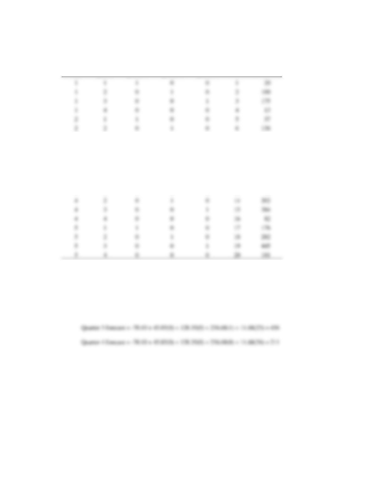
we can use the LINEST function to find the regression model:
Revenue = – 70.10 + 45.03 Qtr1 + 128.35 Qtr2 + 256.68 Qtr3 + 11.68 t
Quarter 1 forecast = -70.10 + 45.03(1) + 128.35(0) + 256.68(0) + 11.68(21) = 221
Quarter 2 forecast = -70.10 + 45.03(0) + 128.35(1) + 256.68(0) + 11.68(22) = 315