Unlock document.
This document is partially blurred.
Unlock all pages and 1 million more documents.
Get Access
6-62.
1
2
3
4
Lead time
SL72
Required
Date
800
1
On-Hand
0
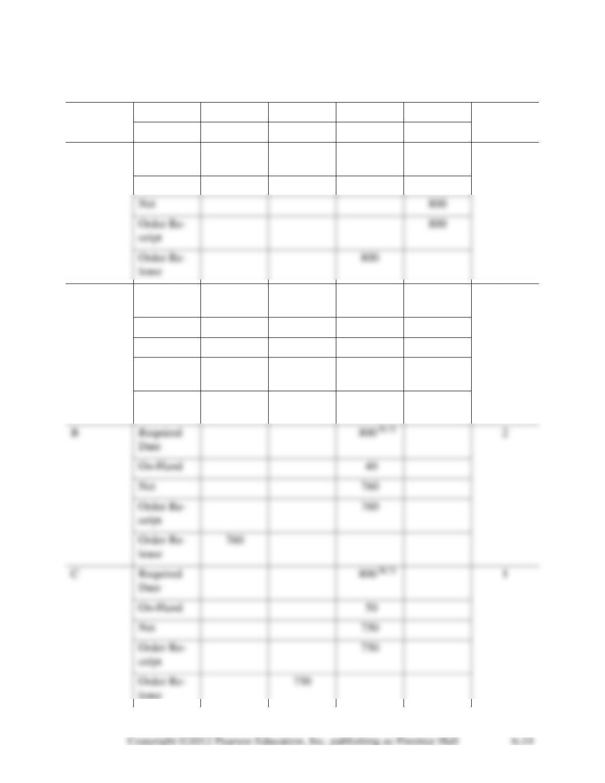
A
Required
Date
800 SL72
1
On-Hand
150
Net
650
Order Re-
ceipt
650
Order Re-
lease
650
E
Required
Date
3000 C
1
On-Hand
0
Net
3000
Order Re-
ceipt
3000
Order Re-
lease
3000
SOLUTIONS TO INTERNET HOMEWORK PROBLEMS
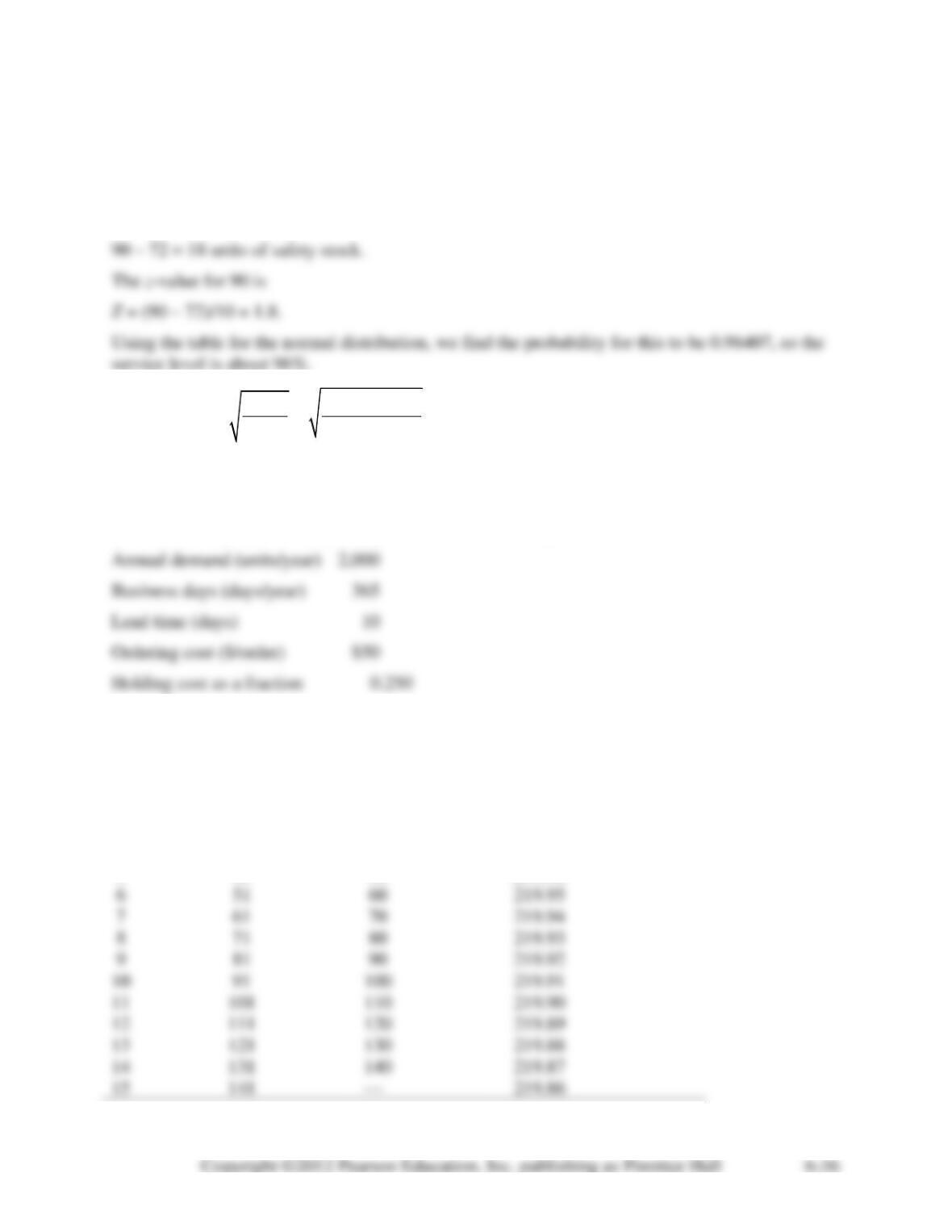
6-63. ROP = mean demand during lead time + safety stock
If ROP = 90, and the average demand during the lead time is 72, then there are
6-64. a.
( )
2 10,000 48
2
EOQ 400
6
o
h
DC
C
= = =
b. safety stock = z
= 1.28(80) = 98.4
c. ROP = 240 + 98.4= 338.4units
6-65. a. The optimal order quantity and the total inventory cost are shown below.
Price
Lower
Upper
Unit
Break
Quantity
Quantity
Price
1
0
10
$220.00
2
11
20
219.99
3
21
30
219.98
4
31
40
219.97
5
41
50
219.96
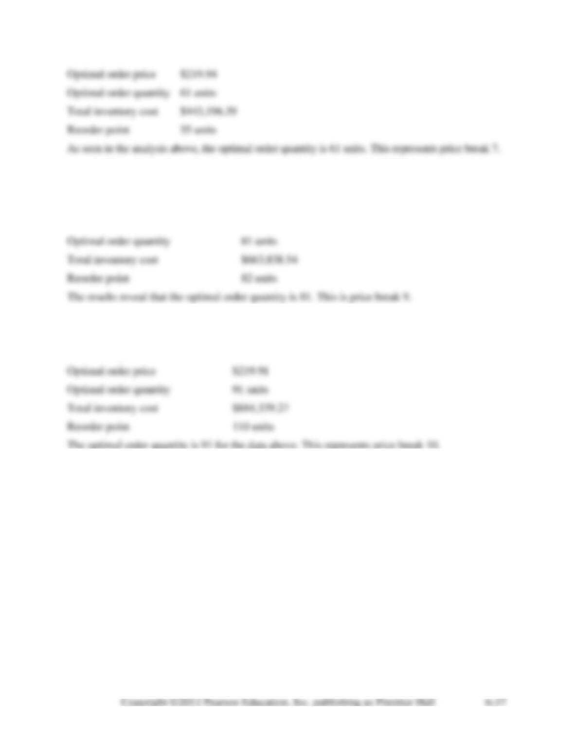
b. The solution for a situation where annual demand is equal to 3,000 is presented below.
Annual demand (units/year)
3,000
All other input is the same.
Optimal order price
$219.92
c. The solution below shows the impact of an increase in annual demand to 4,000 frames:
Annual demand (units/year)
4,000
All other input is the same.
The optimal order quantity is 91 for the data above. This represents price break 10.
d. The optimal order quantity increases and total inventory cost increases. As expected,
higher demand levels allow the ability to take advantage of quantity discounts.
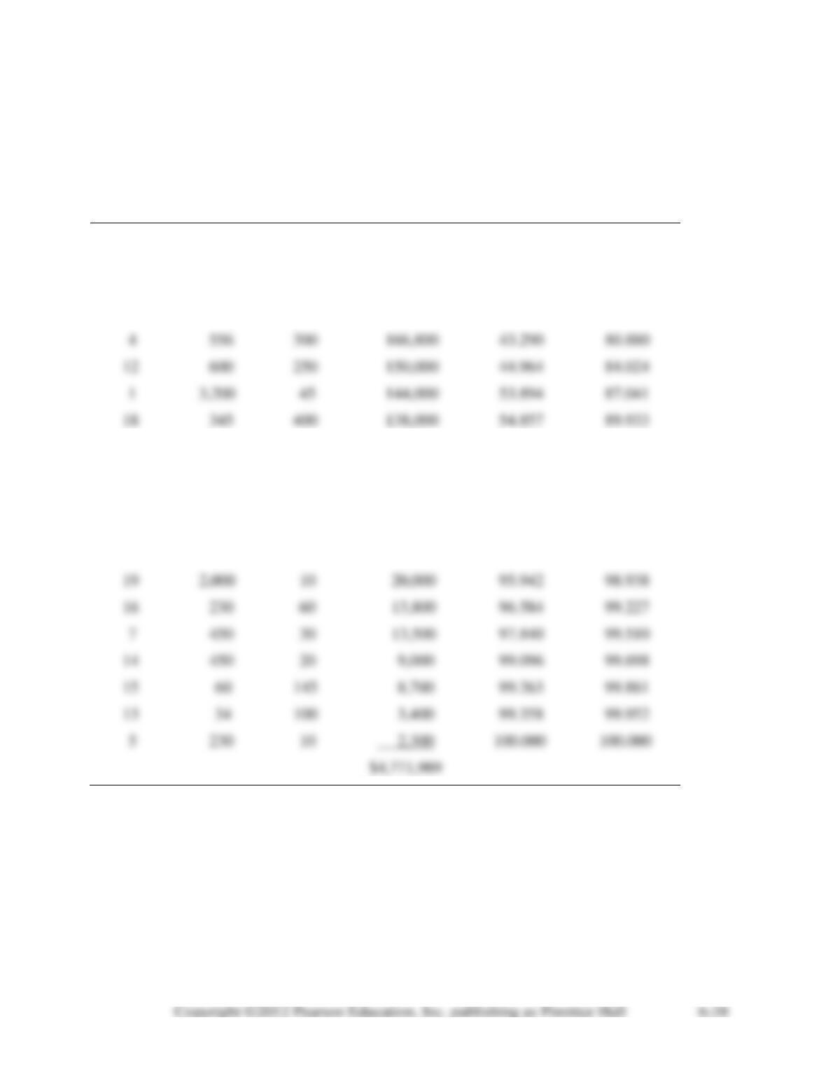
6-66. This is an ABC inventory problem. We can determine the total dollar value of each inven-
tory item. This is shown in the following table:
Annual
Cumulative
Cumulative
Item
Annual
Unit
Dollar
Percentage
Percentage
Number
Demand
Cost
Volume
of Items
of Cost
6
5,600
$400
$2,240,000
15.628
46.941
8
5,400
200
1,080,000
30.698
69.573
11
500
400
200,000
32.093
73.764
9
3,456
50
172,800
41.738
77.385
2
5,543
23
127,489
70.326
92.605
20
5,600
20
112,000
85.954
94.952
17
1,000
100
100,000
88.745
97.047
10
456
100
45,600
90.018
98.003
3
123
200
24,600
90.361
98.518
As you can see, items 6, 8, and 11 represent slightly over 70% total dollar usage. These are A
items, and they should be carefully controlled. Items 9, 4, 12, 1, and 18 represent an additional
20% of total sales. These are B items, and they should be controlled to some extent. The other
items are C items. The stockout data is not needed in this problem. (Item 9 could also be consid-
ered an A item, raising cumulative total $ value to 77%). Rules for breaking A, B, C items into
categories can be flexible and decided by each firm.
6-67. D = 50,000 units; Co = $10; Ch = $4
a.
( )( )
*2 50,000 10 500 units
4
Q==
6-68. D = 50,000 units; Co = $10; Ch = $16
a.
( )( )
*2 50,000 10 250 units
16
Q==
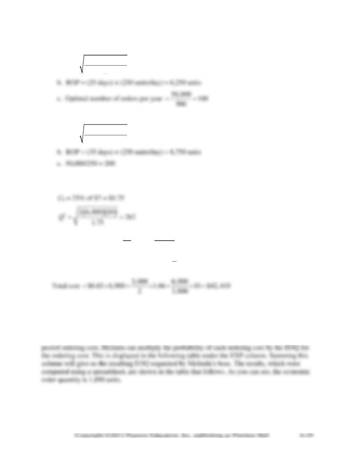
6-69. D = 6,000 units
Co = $10
Total cost
*
*
$6,000
$7 6,000 1.75 10 $42, 458
2
Q
Q
= + + =
If new supplier is used, Ch = 25% of $6.65 ~ $1.66
Q = 3,000
Pampered Pet should use the new supplier and take the discount.
6-70. Melinda can solve this problem by determining the probability distribution for ordering
cost. This is done by finding the total of the frequency of ordering cost and dividing each number
by the total. Melinda can also determine the EOQ value for each possible ordering cost value by
using the equation presented in the chapter. In order to determine the EOQ for the average or ex-
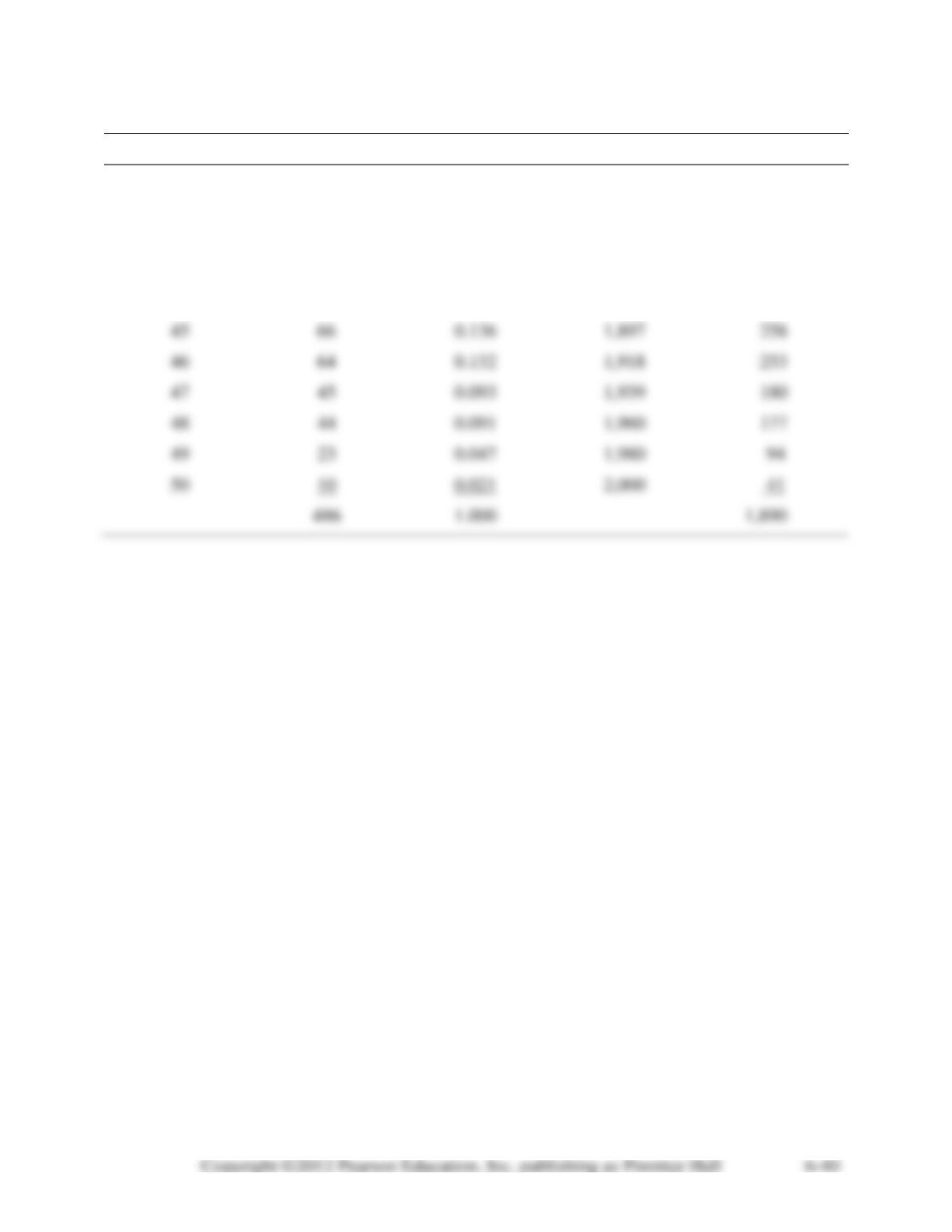
Order Cost
Frequency
Probability
EOQ
EXP
$40
24
0.049
1,789
88
41
34
0.070
1,811
127
42
44
0.091
1,833
166
43
56
0.115
1,855
214
44
76
0.156
1,876
293
SOLUTION TO MARTIN-PULLIN BICYCLE CORPORATION
1. Inventory plan for Martin-Pullin Bicycle Corporation. The forecasted demand is summarized
in the following table.
Jan
Feb
Mar
Apr
May
June
July
Aug
Sept
Oct
Nov
Dec
Total
8
15
31
59
97
60
39
24
16
15
28
47
439
Average demand per month = 439/12 = 36.58 bicycles. The standard deviation of the monthly
demand = 24.58 bicycles.
The inventory plan is based on the following costs and values.
Order Cost = $65/order
The solution below uses the simple EOQ model with reorder point and safety stock. It ignores
the seasonal nature of the demand. The fluctuation in demand is dealt with by the safety stock
based on the variation of demand over the planning horizon.
Economic order quantity (Q*) is given by:
2. The reorder point is calculated by the following relation:
Reorder point (ROP) = average demand during the lead time (
) + z × (standard deviation of
the demand during the lead time (
))
Therefore,
ROP = 36.58 + 1.6425(24.581) 77 bicycles
( ) ( ) ( )
*
1 Total Demand
Holding Cost Holding Cost Ordering Cost
2*
Q ss Q
= + +
= $416.00 + $489.60 + 416.00 = $1321.60
This case can be made more interesting by asking students to trace the inventory behavior with
the above plan (assuming that the forecast figures are accurate and ignoring the forecast errors)
and to see the amount of total stockout, if any. Students then can calculate the lost profit due to
stockout and add it to the total cost.
SOLUTIONS TO INTERNET CASES
LAPLACE POWER AND LIGHT CO.
The optimal order quantity is given by:
( )
*2 499.5 50
2
41.4
DS
QH
==
Currently, the company is committed to take 1/12th of its annual need every month. Therefore,
each month the storeroom issues a purchase requisition for 41,625 feet of cable. With TC = total
inventory cost,
Ordering costs are a linear function because no matter how large an order is or how many orders
are sent in, the cost to order any material is $50 per order.
The student should recognize that it is doubtful the firm will or should alter any current or-
dering policy for a savings of only $23.
WESTERN RANCHMAN OUTFITTERS
The EOQ for a yearly demand of 2,000, order cost of $10.00 and holding cost of 0.12 (10.05) =
$1.206 is
There is one remaining problem which the model doesn’t solve, but which Mr. Randell has.
That is the problem of the unreliability of the supplier. By ordering one extra time (twelve orders
per year instead of eleven) and by ordering extra quantities judiciously, Mr. Randell has man-
aged to keep WRO almost totally supplied with the requisite number of Levi 501s. Further, since
the actual solution is so close to the model solution, and since we have seen that the EOQ is a
robust model, Mr. Veta can feel that he is keeping his inventory goals close to the minimum
while still meeting his goal of avoiding stockouts.
PROFESSIONAL VIDEO MANAGEMENT
1. To determine the reorder points for the two suppliers, daily demand for the videotape systems
must be determined. Since each video system requires two videotape systems that are connected
to it, the demand for the videotape units is equal to twice the number of complete systems.
We will assume that there are 20 working days per month. In other words, there are 5 work-
ing days per week. Making this assumption, we can determine the average daily sales to be equal
to the average monthly sales divided by 20. In other words, the daily sales is equal to 800 units
per day (800 = 16,000/20).
For Kony, the reorder point can be computed in the same manner. Assuming again that there
are 5 working days per week, we can compute the lead time in days. For Kony, it takes 2 weeks
between the time an order is placed and when it is received. Therefore, the lead time in days is
equal to 10 days (10 = 2 × 5). With the lead time expressed in days, we can compute the reorder
point for Kony. This is done by multiplying the lead time in days times the daily demand. There-
fore, the reorder point for Kony is 8,000 (8,000 = 800 × 10).
2. To make a decision concerning which supplier to use, total inventory cost must be considered
for both Toshiki and Kony. Both companies have quantity discounts. Because there are two sup-
3. Each alternative that Steve is considering would have a direct impact on the quantity discount
model and the results. The first strategy is to sell the components separately. If this is done, the
demand for videotape systems could change drastically. In addition to selling the videotape units
DRAKE RADIO
1. In order to figure out the reorder points for the two suppliers, daily demand for the FM tuner
must be derived. Since one FM tuner is required for each DR-2000 (stereo system), demand for
tuners is equal to 1 × (demand for DR-2000).
Assuming that there are 20 working days per month, daily demand can be estimated as fol-
lows:
Avg. Monthly Demand # days/months = Avg. daily demand 800 20 = 40 units
The reorder point is equal to daily demand times the lead time.
ROP = dL
meaning that if Drake Radio is being supplied by Nitobitso, the firm should reorder stock when
the inventory falls to a level of 1,600 units.
2. To make a sound recommendation, total inventory costs for both Collins and Nitobitso must
be determined. Both companies have quantity discounts.
Annual demand is estimated to be 9,600 units (800 units/month × 12 months/yr.).
The first step in determining inventory costs is to determine what the economic order is; then
Nitobitso
( )
( )( )
( )( )
*
2 9,600 100
2577.85
0.25 23
o
DC
QIP
= = =
The lowest total cost for Nitobitso is $207,332.39 with an EOQ of 2,001 units.
A comparison of the two lowest total cost figures indicates that using Nitobitso as supplier
would be the least costly of the two. Ordering costs decreases and price breaks far outweigh any
carrying cost increases in this case.
3. Everything else being equal, Collins would be the best supplier of FM tuners in the event of
fluctuating demand. Collins’ lead time is substantially less than Nitobitso’s. Should high demand


