Chapter 6
7 – 1
Chapter 6
Forecasting
Case Problem 1: Forecasting Food and Beverage Sales
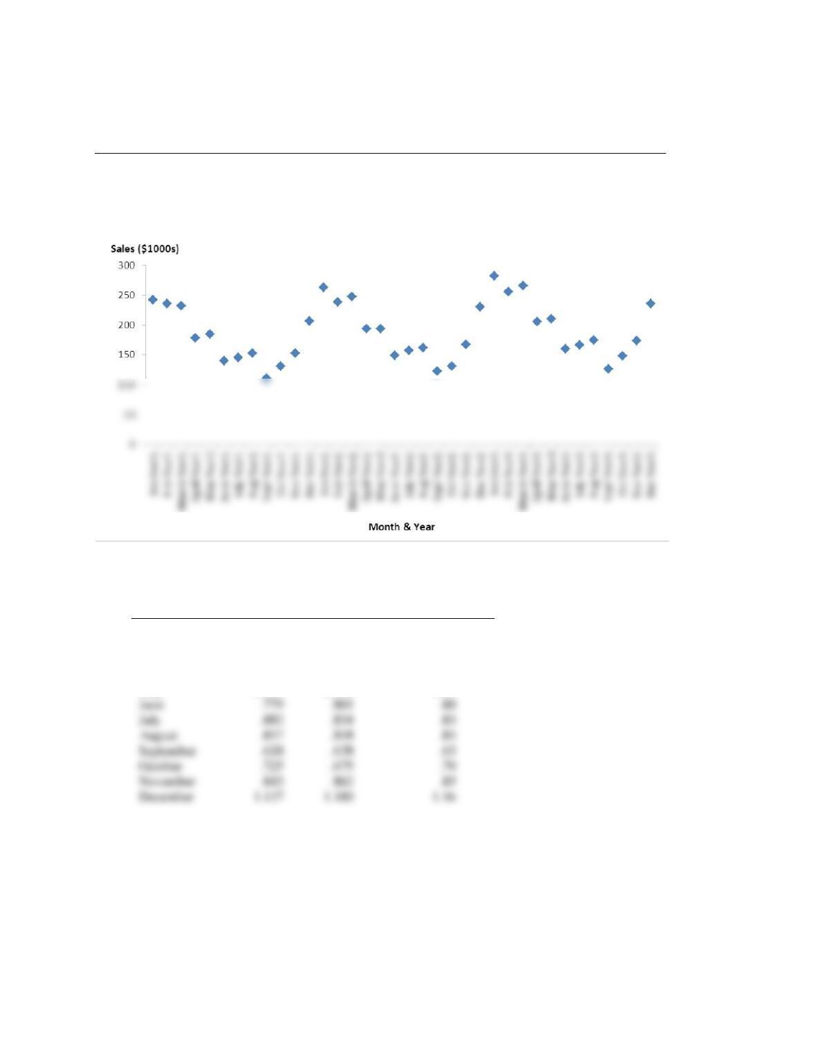
1. Graph of the time series:
2. Analysis of seasonality:
Month
Seasonal-Irregular
Component Values
Seasonal Index
January
1.445
1.441
1.44
February
1.301
1.297
1.30
March
1.344
1.343
1.34
April
1.047
1.034
1.04
May
1.044
1.054
1.05
June
July
August
September
October
November
December
1.137
1.180
1.16

Chapter 6
The deseasonalized time series is shown below:
t
Deseasonalized Sales
t
Deseasonalized Sales
1
168.06
19
189.16
2
180.77
20
189.41
3
173.13
21
193.65
4
171.15
22
185.71
5
175.24
23
196.47
6
175.00
24
198.28
7
174.70
25
195.83
8
178.82
26
196.15
9
174.60
27
197.76
185.71
28
197.12
178.82
29
200.00
177.59
30
200.00
182.64
31
200.00
183.08
32
204.71
184.33
33
200.00
185.58
34
211.43
183.81
35
203.53
186.25
36
202.59
The trend line fitted to the deseasonalized time series is
T t = 169.499 + 1.02 t
3. Sales forecasts
Forecast for Year 4
Using T t = 169.499 + 1.02 t
Month
Trend
Forecast
Seasonal
Index
Monthly
Forecast
January
207.239
1.44
298.424
February
208.259
1.30
270.737
March
209.279
1.34
280.434
April
210.299
1.04
218.711
May
211.319
1.05
221.885
June
212.339
169.871
July
213.359
177.088
August
214.379
182.222
September
215.399
135.701
October
216.419
151.493
November
217.439
184.823
December
218.459
1.16
253.194
4. Forecast error = $295,000 – $298,424 = -$3,424
The forecast we developed over predicted by $3,424; this represents a very small error.
5. The analysis can be easily updated each month, especially if a computer software package is used to
perform the analysis.
Forecasting
6 – 3
Case Problem 2: Forecasting Lost Sales
1. The data used for the forecast is the Carlson sales data for the 48 months preceding the storm. Using the
trend and seasonal method, the seasonal indexes and forecasts of sales assuming the hurricane had not
occurred are as follows:
Month
Seasonal Index
Month
Forecast ($ million)
January
0.957
September
2.16
February
0.819
October
2.54
March
0.907
November
3.06
April
0.929
December
4.60
May
1.011
June
0.937
July
0.936
August
0.974
September
0.797
October
0.936
November
1.119
December
1.677
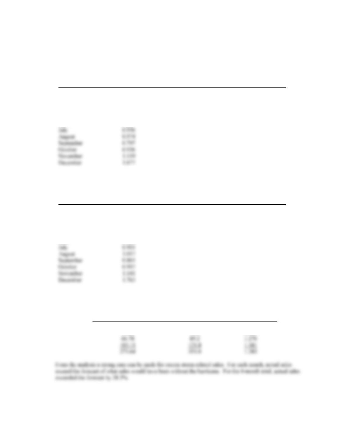
2. The data used for this forecast is the total sales for the 48 months preceding the storm for all department sores
in the county. Using the trend and seasonal method, the seasonal indexes and forecasts of county-wide
department store sales assuming the hurricane had not occurred are as follows:
Month
Seasonal Index
Month
Forecast ($ million)
January
0.773
September
50.55
February
0.813
October
53.20
March
0.976
November
66.78
April
0.935
December
103.11
May
0.989
June
0.924
July
0.901
August
1.017
September
0.861
October
0.907
November
1.141
December
1.763
3. By comparing the forecast of county-wide department store sales with actual sales, one can determine whether or
not there are excess storm-related sales. We have computed a “lift factor” as the ratio of actual sales to forecast
sales as a measure of the magnitude of excess sales.
Forecast Sales ($ million)
Actual Sales ($ million)
Lift Factor
50.55
69.0
1.365
53.20
75.0
1.410
66.78
85.2
1.276
1.181
Chapter 6
6 – 4
4. One approach would be to use the forecast of what sales would have been without the hurricane and then
multiply by the lift factor to account for the excess storm-related sales. Such an estimate of lost sales is
developed below:
Forecast ($ million)
Lift Factor
Lost Sales ($ million)
2.16
1.365
2.948
2.54
1.410
3.581
3.06
1.276
3.905
4.60
1.181
5.433
Total
15.867
Based on this analysis, Carlson Department Stores can make a case to the insurance company for a business
interruption claim of $15,867,000.
Another approach would be to use the 48 months of historical data to compute a market share for Carlson.
That is, compute Carlson’s sales as a fraction of county-wide department store sales. Then you could