Statistical Methods in Quality Management 1
CHAPTER 6
Statistical Methods in Quality Management
Teaching Notes
This chapter describes concepts of statistics, statistical thinking, statistical methodology,
sampling, experimental design, and process capability. Students should be encouraged to take a
big picture perspective on this framework, rather than the approach of: “How do I get the right
answer?”
Although this chapter reviews many of the basic concepts and techniques of statistics that
are relevant to the technical areas of statistical process control (SPC), it is by no means
comprehensive. Students should be encouraged to consult a statistics textbook for further
insights on the topics in this chapter. These topics are typically covered in business or
engineering statistics course that students should have had prior to taking a course using this text.
Key objectives for this chapter include:
• To establish the importance of statistics as the “bridge” between quality of design and
quality of conformance. The proper use of statistics is highlighted as a quality
improvement tool.
• To help students appreciate the importance of statistical thinking in order to understand
inter-related processes, process variation, and the need to reduce it in order to assure
quality in operations.
ANSWERS TO QUALITY IN PRACTICE FEATURES
Modern Applications of Statistics in Quality
Key Issues for Discussion
Statistical Methods in Quality Management 2
1. Why should statistics be taught to, and understood by, employees in all functions and all
levels of an organization?
Statistics should be taught to, and understood by, employees in all functions and all levels of an
organization because statistics is the foundation for quality design, improvement, and control.
2. Summarize and classify the numbered examples (6.1 through 6.24) in this chapter by
type of statistical application in quality based on the ideas in this Quality in Practice
feature. In other words, does the example illustrate application in product design,
reliability, manufacturing, service, and so on?
The numbered examples [6.1 – 6-24] in this chapter have been classified by type of statistical
application in quality based on the ideas in this Quality in Practice feature. They have also been
Example No. Name Function Industry
EX. 6.1 Using Probability Rules Process Improvement Computers
EX. 6.2 Applying Conditional Probability Product Design and Reliability Multiple
EX. 6.3 Multiplication Rule – Indep. Events Process Improvement Multiple
EX. 6.4 Using the Binomial Distribution Process Improvement Multiple
EX. 6.5 Using the Poisson Distribution Manufacturing Multiple
EX. 6.6 Using the Normal Distribution Product Design and Reliability Medical

Statistical Methods in Quality Management 3
EX. 6.16 Computing a CI Stdev Unknown Product Design and Reliability Medical
EX. 6.17 Computing a CI for a Proportion Product Design and Reliability Service
EX. 6.18 Hypothesis Test for the Mean Product Design and Reliability Software
EX. 6.19 Using Excel Hypothesis Tools Product Design and Reliability Multiple
Improving Quality of a Wave Soldering Process Through the Design of Experiments
1. Why did the first experimental design not find the true optimum combination of factors
to achieve the maximum reduction of defects?
The first experimental design at the HP plant did not achieve the true optimum combination of
factors, because not all combinations were tested. It is theoretically possible that a better
2. What were some of the advantages of using experimental design over a traditional trial–
and-error approach?
Experimental design allows the experimenter to systematically evaluate two or more methods to
determine which is better, or to determine the levels of controllable factors to optimize process
ANSWERS TO REVIEW QUESTIONS
1. What is the science of statistics? Why is it important in quality management?
Statistics is a science concerned with “the collection, organization, analysis, interpretation, and
Statistical Methods in Quality Management 4
presentation of data.” Statistics is essential for quality and for implementing a continuous
2. Explain the difference between an experiment, an outcome, and a sample space.
In statistical terminology, an experiment is a process that results in some outcome. The outcome
of an experiment is a result that we observe. The collection of all possible outcomes of an
3. State the four rules for calculating probabilities of events.
The following rules apply to calculating probabilities of events:
Rule 1: The probability of any event is the sum of the probabilities of the outcomes that compose
that event.
Rule 2: The probability of the complement of any event A is P(Ac) = 1 – P(A).
4. Explain the multiplication rule of probability. How does independence of events affect
the multiplication rule?
The multiplication rule of probability is: P(A and B) = P(A | B) P(B) = P(B | A) P(A), where P(A |
B) reads as the conditional probability of A, given B. Conditional probability is the probability of
5. List the most important types of probability distributions used in quality management.
The two most important types of probability distributions are discrete and continuous
distributions. Under the discrete category, the binomial and Poisson distributions are the most
important. The binomial distribution calculates the probability of exactly x successes in a
Statistical Methods in Quality Management 5
probability density function, and is described by a mathematical function f(x). For continuous
random variables, it does not make mathematical sense to attempt to define a probability for a
specific value of x because there are an infinite number of values.
Sample statistics such as , s, and p are random variables that have their own
6. How do discrete probability distributions differ from continuous probability
distributions?
A probability distribution can be either discrete or continuous, depending on the nature of the
random variable it models. For discrete probability distributions, a complete, finite number of
outcomes and their associated probabilities of occurrence can be listed. These outcomes are
called a list of mutually exclusive and collectively exhaustive outcomes.
A continuous random variable is defined over one or more intervals of real numbers, and
therefore, has an infinite number of possible outcomes. A curve that characterizes outcomes of a
continuous random variable is called a probability density function, and is described by a
mathematical function f(x). For continuous random variables, it does not make mathematical
sense to attempt to define a probability for a specific value of x because there are an infinite
number of values. Probabilities are only defined over intervals.
7. List and explain the three basic elements of statistical methodology.
The three basic elements of statistical methodology are descriptive statistics, statistical inference,
and predictive statistics. The methods for the efficient collection, organization, and description of
data are called descriptive statistics. Statistical inference is the process of drawing conclusions
about unknown characteristics of a population from which the data were taken. Predictive
statistics is used to develop predictions of future values based on historical data. The three differ
in approach, purpose, and outcomes. Descriptive statistics simply summarize and report on
Statistical Methods in Quality Management 6
8. Describe the common types of sampling schemes.
Methods of sample selection, or sampling schemes, include: simple random sampling, stratified
sampling, systematic sampling and cluster sampling. Simple random sampling is useful where
one needs to gather information from a moderately large, homogeneous population of items. For
example, if a MBA director wished to find out the attitudes of 300 MBA students toward various
policies, procedures, and services provided to the students, s(he) might use a simple random
9. What is the difference between sampling error and systematic error? Why are these
important to understand?
Any sampling procedure can result in two types of errors: sampling error and systematic error.
Sampling error occurs naturally and results from the fact that a sample may not always be
representative of the population, no matter how carefully it is selected. The only way to reduce
sampling error is to take a larger sample from the population. Systematic errors, however,
usually result from poor sample design and can be reduced or eliminated by careful planning of
the sampling study.
10. Explain the difference between a population and a sample.
A population is a complete set or collection of objects of interest. A sample is a subset of objects
taken from a population.
11. List the common types of statistical measures of location and explain how to compute
them.
Measures of location are essentially those that focus on central tendency, such as the mean,
median, and mode. The mean is the average, the median is the point above and below which 50
Statistical Methods in Quality Management 7
percent of the values of a sample or population fall, and the mode is the most commonly
occurring value.
12. List the common types of statistical measures of dispersion and explain how to compute
them.
13. Explain how to compute a proportion.
The proportion, usually denoted as p, is used to measure the fraction of data that have a certain
characteristic. For example, the fraction of respondents that is female or male. Proportions are
key descriptive statistics for categorical data, such as defects or errors. Such categorical data are
not numerical, but rely on counting items that fall into categories of interest. Thus, statistics such
as means and variances are not appropriate, where proportions are involved.
14. Explain the difference between the standard deviation and the standard error of the
mean. How are they related?
The standard error of the mean is the (estimated) standard deviation of the population divided
by
n
or ( /
n
). The standard deviation is, of course, a measure of variability within a
15. State the meaning of the central limit theorem in your own words. How important is it
to the development and use of statistical quality control techniques?
The central limit theorem is extremely useful in that it states (approximately) that a sampling
distribution can be defined as the distribution obtained by taking a large number of samples of
n
16. What are some of the descriptive statistical tools available in Microsoft Excel, and how
can they be used?
Microsoft Excel provides data analysis tools, called the Analysis ToolPak, that are useful in
complex statistical analyses. You provide the data and parameters for each analysis; the tool uses
the appropriate statistical functions and then displays the results in an output table. Some tools
Statistical Methods in Quality Management 8
17. What is a confidence interval? What value do they have?
A confidence interval (CI) is an interval estimate of a population parameter that also specifies the
likelihood that the interval contains the true population parameter. This probability is called the
level of confidence, denoted by 1 – , and is usually expressed as a percentage. Used together,
these statistical tools can help clarify what we know and don’t know about a population, based
18. Describe some applications of hypothesis testing that might be applied to the topics in
Chapters 3, 4, and 5.
Some applications of hypothesis testing that might be applied to the topics in Chapters 3, 4, and
5 are varied. For example, a hypothesis might be tested concerning the question of whether
customers are more likely to prefer one brand over another, for similar products, in Chapter 3. In
19. Explain the hypothesis that is tested in analysis of variance.
ANOVA is a methodology for drawing conclusions about equality of means of multiple
populations. In its simplest form – one-way ANOVA – it compares means of observed responses
of several different levels of a single factor. ANOVA tests the hypothesis that the means of all
populations are equal against the alternative hypothesis that at least one mean differs from the
others.
20. Explain the concepts of correlation and regression.
Correlation is a measure of a linear relationship between two variables, X and Y, and is measured
by the (population) correlation coefficient. Correlation coefficients will range from -1 to +1. A
correlation of 0 indicates that the two variables have no linear relationship to each other. Thus, if

Statistical Methods in Quality Management 9
21. What is the purpose of design of experiments?
The purpose of design of experiments is to set up a test or series of tests to enable the analyst to
compare two or more methods to determine which is better, or to determine levels of controllable
factors to optimize the yield of a process, or minimize variability of a response variable.
22. Describe a factorial experiment. Provide some examples of factorial experiments that
you might use to solve some type of quality-related problem.
A factorial experiment is a specific type of experimental design that considers all combinations
SOLUTIONS TO PROBLEMS
1. A new production process at Fabufirst, Inc., has two in-line stages. The probability of
defective components being produced in stage 1 is 15 percent and 10 percent in stage 2.
Assembled units that have defective components only from stage 1 OR only from stage 2
are considered repairable. However, items that have defective components from both stage
1 and stage 2 (completely defective) must be scrapped.
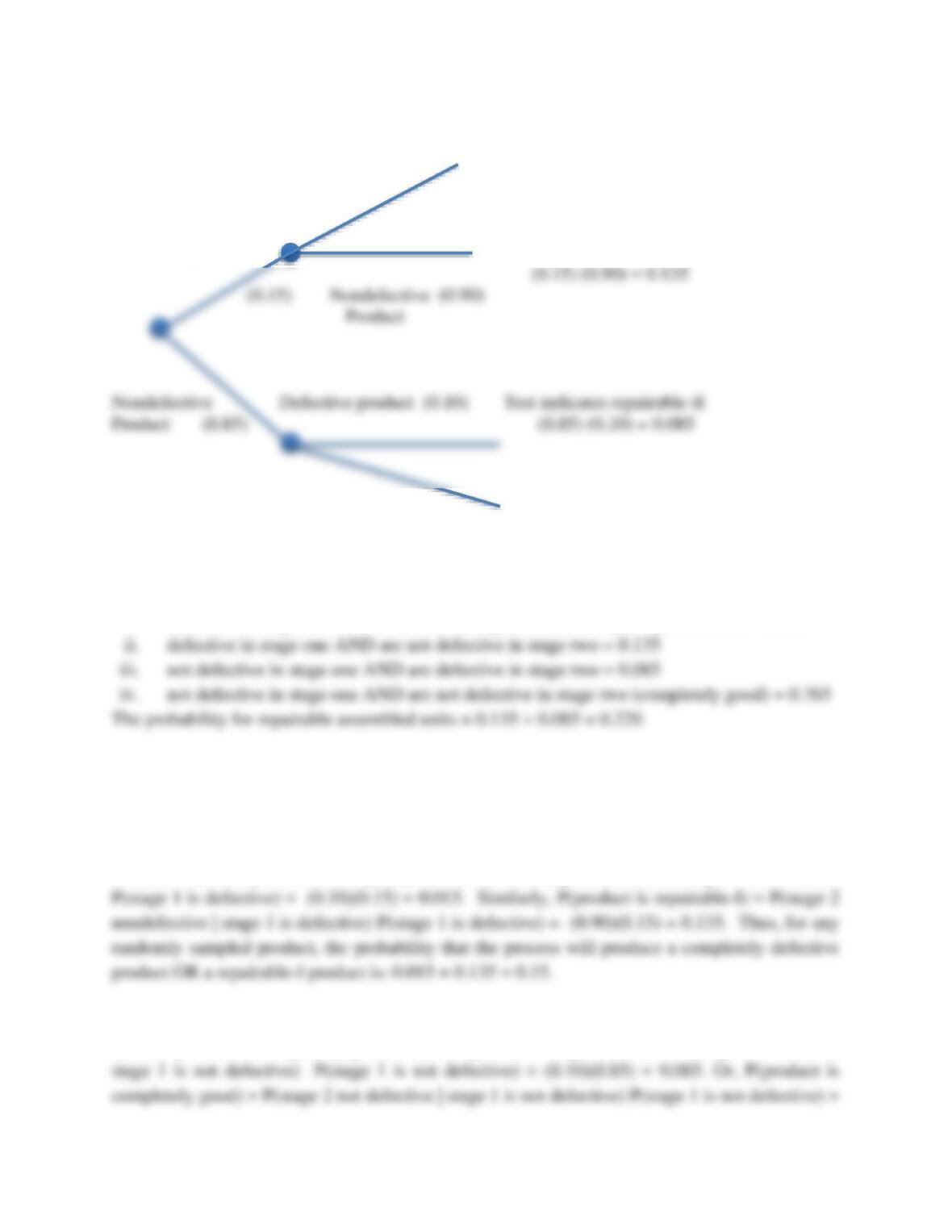
a. Use a probability tree diagram and calculate the probabilities that the Fabufirst
assembled units are: (i) defective in stage 1 and defective in stage 2 (are completely
defective); (ii) defective in stage 1 and are not defective in stage 2 (called Repairable I); (iii)
not defective in stage 1 but are defective in stage 2 (called Repairable II); and (iv) not
defective in stage 1 and are not defective in stage 2 (completely good). What is the
probability of producing repairable assembled units?
Statistical Methods in Quality Management 10
Test indicates completely defective
(0.15) (0.10) = 0.015
Defective product (0.10)
Defective product Test indicates repairable-I
Nondefective (0.90) Test indicates completely good
Product (0.85) (0.90) = 0.765
As shown on the tree diagram, the probabilities that the Fabufirst units are:
i. defective in stage one AND defective in stage two (are completely defective) = 0.015
b. Explain the results in terms of the multiplication and the addition rules for probability.
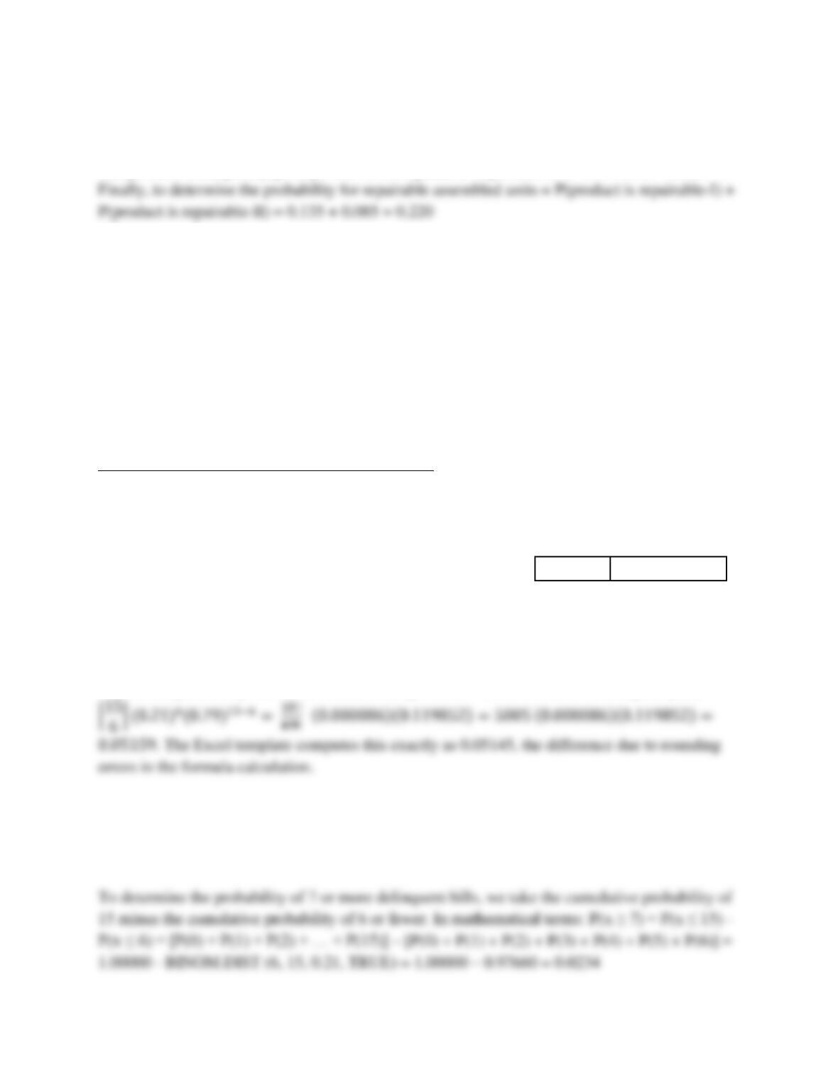
Using the multiplication rule, the probability that any Fabufirst product coming off the assembly
line is completely defective can be found by multiplying the probabilities along the branches of
the tree. Thus, P(product is completely defective) = P(stage 2 defective | stage 1 is defective)
We may also compute the conditional probability that the product is defective, but repairable, or
that the product is completely good. Thus, P(product is repairable-II) = P(stage 2 defective |
Statistical Methods in Quality Management 11
(0.90)(0.85) = 0.765 . Thus, for any randomly sampled product, the probability that the process
will produce a completely good product OR a repairable-II product is: 0.765 + 0.085 = 0.85.
2. Auditors at the Valles Verdes Partners, P.S.C. took a sample of 150 accounts payable
bills, as shown in the table found in the Excel worksheet Prob. 6-2 in the Excel workbook
C06Data.
a. Find the proportion of the accounts payable in the sample that are classified as overdue
by using the Excel COUNTIF function.
b. If an auditor takes a random sample of only 15 accounts from this population, assuming
that they follow a binomial distribution, what is the probability that: (i) exactly 6 bills will
be overdue? (ii) 3 or fewer bills will be overdue? (iii) 7 or more bills will be overdue? Use
the binomial probability distribution formula and verify your result using Excel Binomial
spreadsheet template.
See the instructor’s Excel solution file Problem 6.2
a. The output shows:
TRUE
FALSE
COUNTIF (RANGE, CRITERIA) —> COUNTED ITEMS
32
118
PERCENT OF TOTAL
21 percent
79 percent
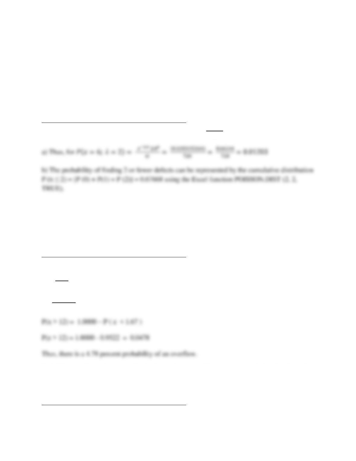
b. The binomial distribution’s function has this form: 𝑓(𝑥)=[𝑛
𝑥](𝑝)𝑥(1−𝑝)𝑛−𝑥
To find the probability that 6 bills within a sample of 15 will be overdue, we compute: 𝑓(6)=
The probability of 3 or fewer bills being overdue is P (x ≤ 5) = P (0) + P(1) + P (2) + P(3).
Rather than calculating individual terms, the Excel BINOM.DIST (5, 15, 0.21, TRUE) calculates
the cumulative probability of 0.61046.
Statistical Methods in Quality Management 12
3. The Turkalike Rug Company buys medium grade carpet in 100-foot rolls. The average
number of defects per roll is 2.0. Assuming that these data follow a Poisson distribution,
use the Poisson spreadsheet template to answer the following questions.
a) What is the probability of finding exactly 6 defects in a carpet roll chosen at random?
b) What is the probability of finding 2 or fewer defects in a carpet roll?
See the instructor’s Excel solution file Problem 6.3.
The Poisson distribution’s function has this form: 𝑓(𝑥)= 𝒆−𝝀 𝝀𝒙
𝒙!
4. Rainbow Punch was made by Frutayuda, Inc. and sold in 12-ounce cans to benefit
victims of Hurricane Zero. The mean number of ounces placed in a can by an automatic fill
pump is 11.7 with a standard deviation of 0.18 ounce. Assuming a normal distribution,
determine the probability that the filling pump will cause an overflow in a can, that is, the
probability that more than 12 ounces will be released by the pump and overflow the can.
See the instructor’s Excel solution file Problem 6.4.
The mean, µ = 11.7; the standard deviation, = 0.18
z = 𝑥− 𝜇
𝜎
z = 12− 11.7
0.18 = 1.67
5. El Grande Green Tea is sold in 350 milliliter cans. The standard deviation for the filling
process is 9 milliliters. What must the target mean for the process be to ensure that the
probability of overfilling more than 350 ml in a can is at most 1 percent?
See the instructor’s Excel solution file Problem 6.5.
Statistical Methods in Quality Management 13
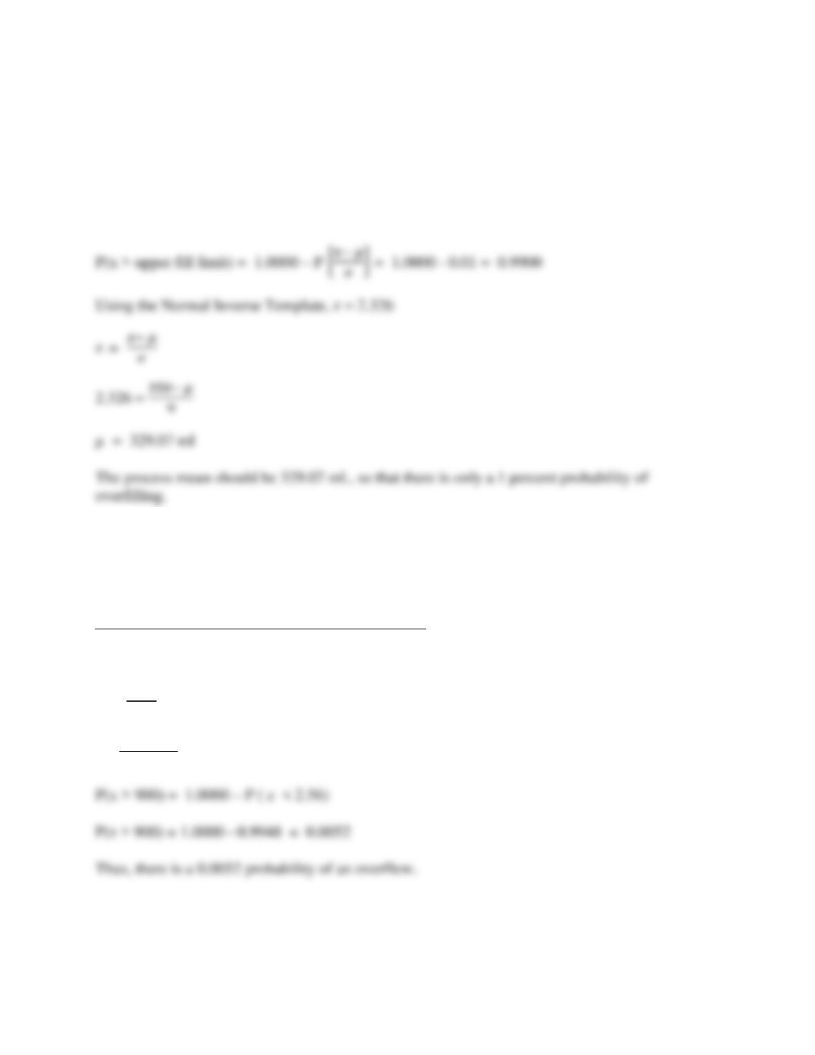
The values for the 1 percent cutoff and the standard deviation are:
x = 350 ml; = 9 ml
For a total probability of 1 percent for overfilling:
6. Frackly Oil is sold in 900 milliliter (ml) cans. The mean volume of oil placed in a can is
880 ml with a standard deviation of 7.8 ml. Assuming a normal distribution of the data,
what is the probability that the filling machine will cause an overflow in a can, that is, the
probability that more than 900 ml will be placed in the can?
See the instructor’s Excel solution file Problem 6.6.
The mean is µ = 880; the standard deviation, = 7.8, x = 900.
z = 𝑥− 𝜇
𝜎
z = 900− 880
7.8 = 2.56
7. Sparkly Cleaning Co. has found that standard size offices have a standard deviation of 5
minutes for their cleaning time. The operations manager knows that 95 percent of the
Statistical Methods in Quality Management 14
offices require more than 120 person-minutes to clean. However, she wishes to find out the
average cleaning time for the offices. Can you calculate that for her?
See the instructor’s Excel solution file Problem 6.7.
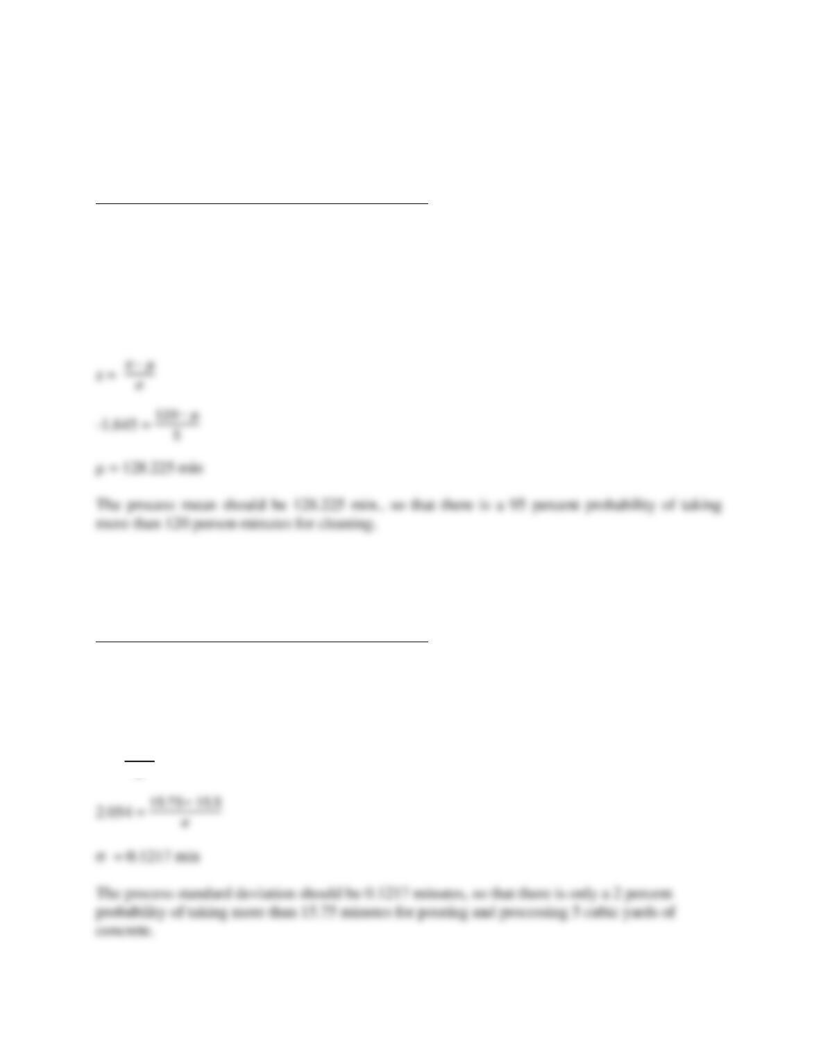
Given that the standard deviation is = 5 min., x = 120, and P (z > x) = 0.95. Using the
NORM.INV function, we have to solve for z when:
P (z < x) = 0.05
Using the Normal Inverse Template, z = -1.645
8. The mean time to pour and process 5 cubic yards of concrete by the Ohio Valley
Construction is 15.5 minutes. If 2 percent of the projects with 5 yards of concrete require
more than 15.75 minutes, what is the standard deviation of the time for such projects?
See the instructor’s Excel solution file Problem 6.8.
Given that the mean process time is µ = 15.5 minutes for the standard pour of 5 cubic yards of
concrete, we find z by taking P (z < x) = P(1.0000) – P (0.0200) = 0.9800. Using the Normal
Inverse template with p = 0.98, z = 2.054.
z = 𝑥− 𝜇
𝜎
Statistical Methods in Quality Management 15
9. The dimension of a machined part made by Perfection Machining, Inc. has a nominal
specification of 7.6 cm. The process that produces the part can be controlled to have a
mean value equal to this specification, but has a standard deviation of 0.3 cm. What is the
probability that a part will have a dimension:
a) exceeding 8.1 cm?
b) between 7.6 and 7.95 cm?
c) less than 7.25 cm?
See the instructor’s Excel solution file Problem 6.9.
The mean value for the machined part in cm is: µ = 7.6; the standard deviation, = 0.3
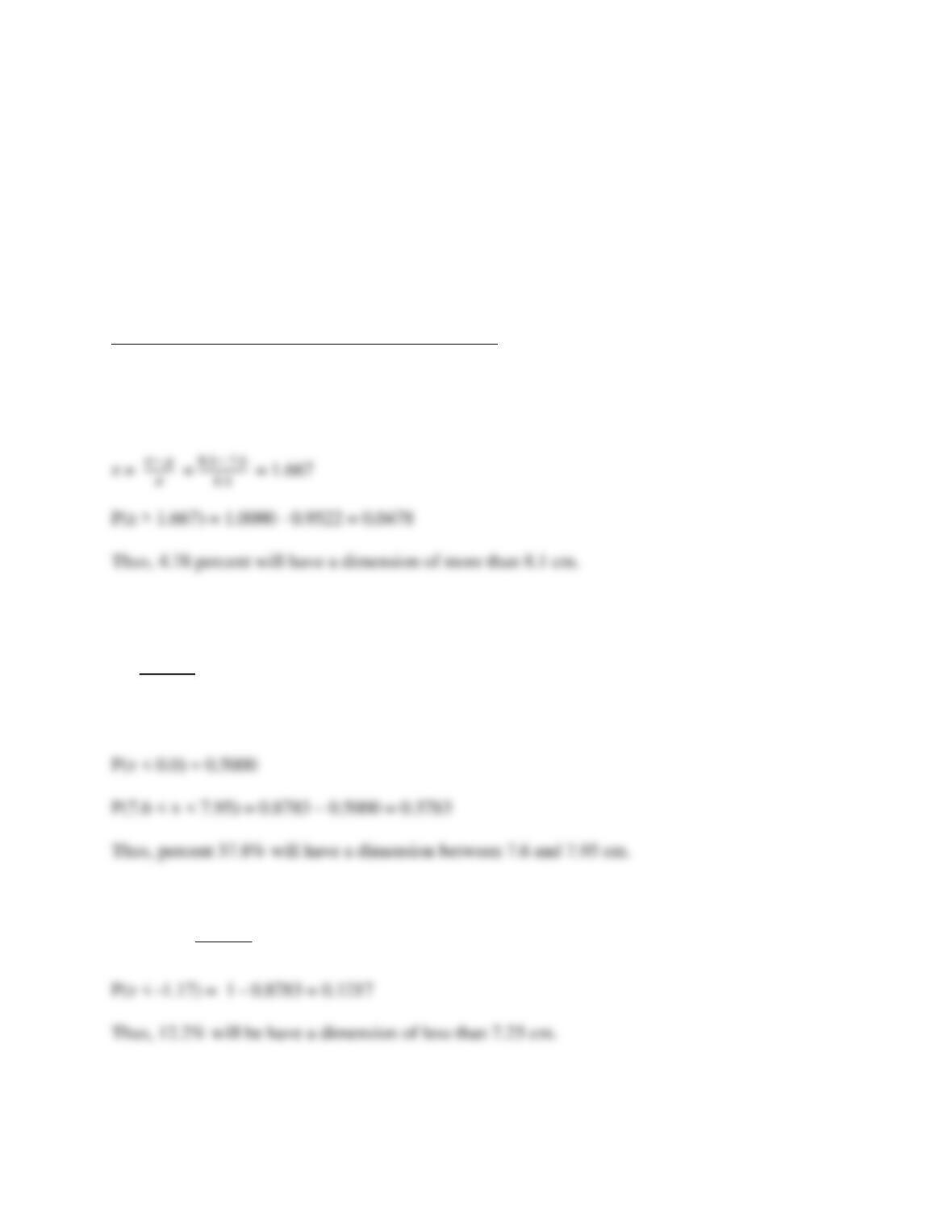
a) P(x > 8.1 cm) = 1.0000 – P ( x < 8.1)
b) P(7.6 < x < 7.95) = P(x < 7.95) – P(x < 7.60)
z = 7.95− 7.6
0.3 = 1.167
P(z < 1.17) = 0.8790
c) For P(x < 7.25)
z = 7.25− 7.6
0.3 = -1.167
10. Genjeteye, Inc. makes aircraft engines. The mean time to failure has been found to be
100,000 hours and is exponentially distributed.
Statistical Methods in Quality Management 16
a) What is the failure rate, , per hour?
b) What is the cumulative probability of failure after 10,000 hours or fewer? Between
10,000 and 15,000 hours?
c) If Genjeteye wishes to provide a warranty that no more than 5 percent of the units will
fail, how many hours of operation without failure should the company guarantee?
See the instructor’s Excel solution file Problem 6.10.
a) 𝜆= 1
𝑀𝑇𝑇𝐹= 1
100,000=0.00001
b) The cumulative probability function is: 𝐹(𝑥)= 1 − 𝑒− 𝜆𝑥
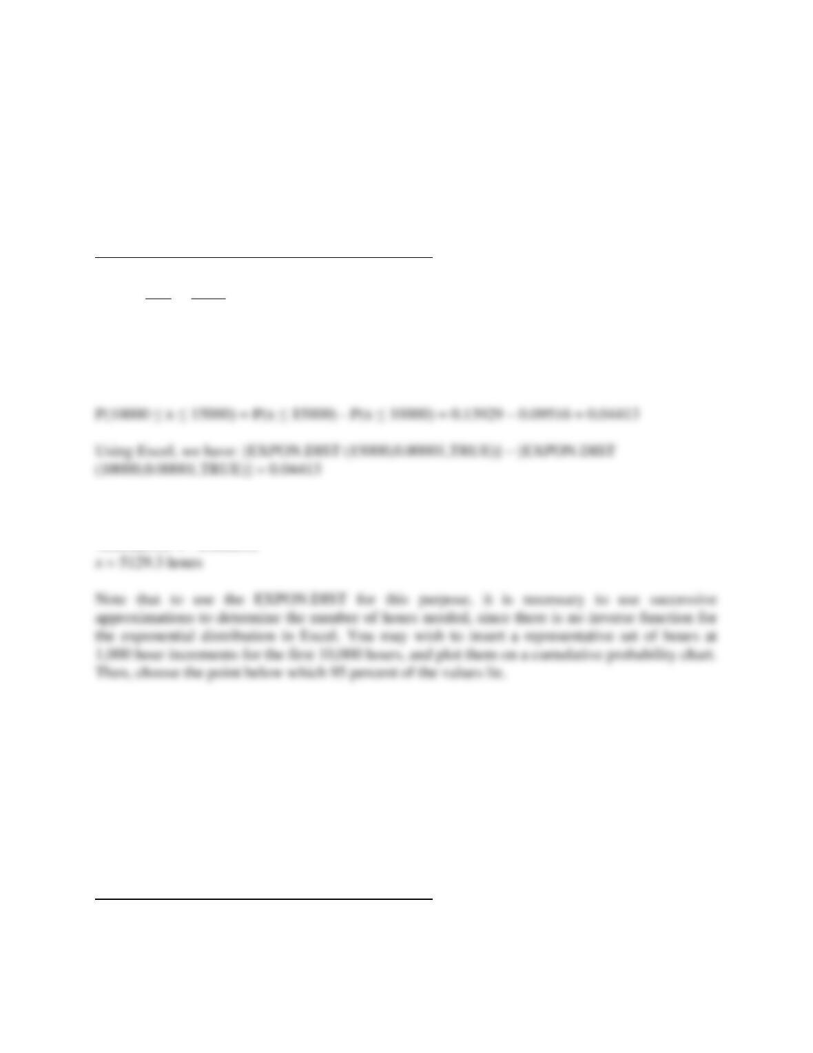
P(x ≤ 10000) = EXPON.DIST(10000, 0.00001,TRUE) = 0.09516
c) For a cumulative P(x) ≤ .05 = 1 − 𝑒− 𝜆𝑥=1 − 𝑒− 0.00001𝑥; Thus, 0.95=𝑒− 0.00001𝑥
Taking natural logs of both sides, we have: ln(0.95) = – 0.00001x
-0.05129.33 = – 0.00001x
11. Use the data for Twentyfirst Century Laundry for the weights of loads of clothes
processed through their washing department in a week. (See Prob. 6-11 in C06Data
workbook).
a. Apply the Excel Descriptive Statistics tool to compute the mean, standard deviation, and
other relevant statistics, and interpret the results in a meaningful fashion.
b. Use the Frequency Distribution and Histogram Excel template to construct a frequency
distribution and histogram for the data. From what type of distribution might you suspect
the data are drawn? Experiment with the number of cells to create a visually-appealing
histogram and use the Excel Histogram tool to verify the results.
See the instructor’s Excel solution file Problem 6.11.
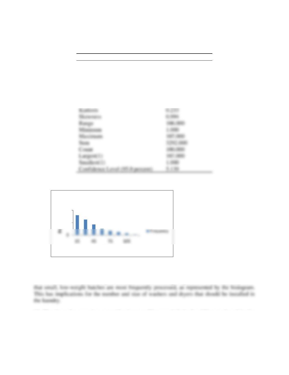
The following results were obtained from the Twentyfirst Century Laundry data
Statistical Methods in Quality Management 17
Descriptive Statistics
Mean
32.920
Standard Error
2.590
Median
25.500
Mode
14.000
Standard Deviation
25.899
Sample Variance
670.741
The conclusion that can be reached from looking at the summary statistics and the histogram is
that these data are exponentially distributed, with descending frequencies. These data may show
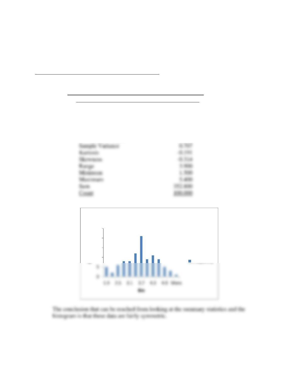
12. The times for carrying out a blood test at Rivercreek Labs for 100 tests, found in the
Prob. 6-12, in the C06Data Excel workbook, were studied in order to better understand the
process. Apply the Descriptive Statistics tool to compute summary statistics and explain the
20
40
Bin
Histogram
Kurtosis
0.233
Skewness
0.994
Range
106.000
Minimum
1.000
Maximum
107.000
Sum
3292.000
Count
100.000
Largest(1)
107.000
Smallest(1)
1.000
Confidence Level (95.0 percent)
5.139
Statistical Methods in Quality Management 18
results. Also, construct a frequency distribution and histogram, for the data taken from
set.
See the instructor’s Excel solution file Problem 6.12.
Students may use different bins in constructing the histogram.
Descriptive Statistics
Mean
3.528
Standard Error
0.084
Median
3.600
Mode
4.100
Standard Deviation
0.841
13. The data for Prob. 6-13 found in C06Data Excel workbook shows the weight of a set of
castings (in kilograms) being made in the Fillmore Metalwork foundry. Construct an Excel
10
15
20
25
Histogram
Frequency
Sample Variance
0.707
Kurtosis
Skewness
Range
3.900
Minimum
1.500
Maximum
5.400
Sum
Count
Statistical Methods in Quality Management 19
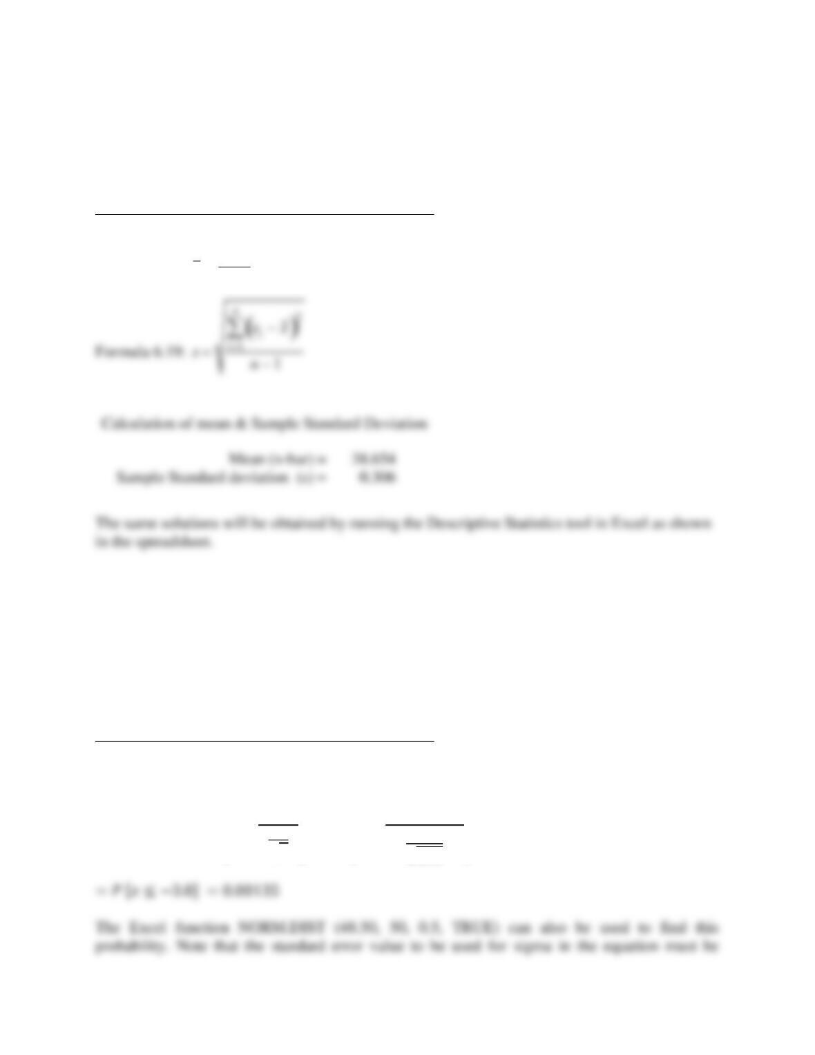
spreadsheet to compute the mean and the sample standard deviation using formulas (6.15)
and (6.19). Verify your results using Excel functions.
See the instructor’s Excel solution file Problem 6.13.
Formula 6.15:
14. A warehouse manager at Dockhousing, Inc. maintains a large inventory of video games.
The company’s database states that the mean value of the games in inventory is $50, with a
standard deviation of $5. The manager is concerned about pilfering the more expensive
games by the warehouse employees. She picked a random sample of 100 games and found
the mean value to be $48.50. Assuming a normal distribution, what is the probability that
the sample mean would be $48.50 or less, if all the inventory can actually be accounted for?
What conclusions would you reach?
See the instructor’s Excel solution file Problem 6.14.
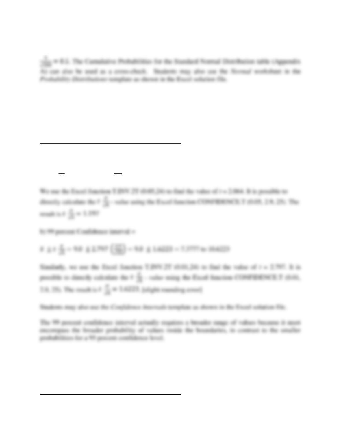
a) Since this probability is on the lower tail of the normal distribution, we must calculate:
𝑃[𝑥≤48.50]= 𝑃[𝑧≤𝑥−𝜇
𝜎
√𝑛] = 𝑃 [𝑧≤48.50−50
5
√100 ]
x=
xi
i=1
n
n
Statistical Methods in Quality Management 20
5
15. The distribution center manager at internet distributor Plastik Parts Warehouse wants
to find a confidence interval for the average time required for an associate to fill an order
for shipment. A sample of 25 orders is taken and the mean time was found to be 9.0
minutes, with a standard deviation of 2.9 minutes. Compute 95 percent and 99 percent
confidence intervals. Which one is larger? Explain why.
See the instructor’s Excel solution file Problem 6.15.
a) 95 percent Confidence interval =
𝑥̅ ± 𝑡 𝜎
√𝑛=9.0 ± 2.064 (2.9
√25)=9.0 ± 1.197= 7.803 to 10.197
16. A new product is being tested by Zed Electronics to determine if it will continue to
operate in a stable fashion under a variety of conditions. A sample of 400 items were tested,
and 60 failed the test. Determine a 90 percent confidence interval for the population
proportion.
See the instructor’s Excel solution file Problem 6.16.