CHAPTER 6
Inventory Control Models
TEACHING SUGGESTIONS
Teaching Suggestion 6.1: Importance of Inventory Control.
Inventory control is important to most organizations. This chapter on inventory control can be
introduced to students by a discussion of the consequences of too much and not enough invento-
Teaching Suggestion 6.2: Examples of the Functions of Inventory Control.
The importance of inventory to store resources, take advantage of quantity discounts, and avoid
Teaching Suggestion 6.3: Importance of Basic Inventory Assumptions.
The assumptions of the basic EOQ model are important. The simple EOQ formula is a direct re-
sult of these assumptions. Students can be told that these assumptions will be relaxed in more
complex models and inventory procedures.
Teaching Suggestion 6.4: Setting Ordering Cost Equal to Carrying Cost Doesn’t Always Work
for More Complex Models.
This chapter determines the formula for the basic economic order quantity by setting ordering
Teaching Suggestion 6.5: Other Ways of Looking at Inventory Problems.
In this chapter, students are shown how to compute the optimal number of orders per year and
the number of days between orders. This was done so students can see that there are different
Teaching Suggestion 6.6: Comparing the Basic EOQ Model with the EOQ Model without the
Instantaneous Receipt Assumption.
This chapter computes EOQ for the case where the instantaneous receipt assumption is relaxed.
A comparison of the traditional EOQ model and this model can be made. The major difference is
Teaching Suggestion 6.7: Adjusting the Order Quantity Upward.
The quantity discount model is not difficult to apply. The major problem students have is that
they forget to adjust the order quantity upward if the quantity is too low to qualify for the dis-
Teaching Suggestion 6.8: Stockout Cost Calculations May Be Difficult to Understand for Some.
The safety stock calculations with known stockout costs is straightforward. The only area that
Teaching Suggestion 6.9: High Cost of a High Service Level.
The computations for stockout policy without stockout costs are easy to understand. The analysis
assumes that demand follows a normal distribution. Students should be told that the same type of
analysis can be made with other probability distributions. It is even possible to perform this type
of analysis with an observed discrete probability distribution.
Teaching Suggestion 6.10: Use of ABC Analysis.
ABC analysis is a very practical and useful concept. Although the mathematics is straightforward
and easy to understand, these techniques can result in substantial savings. Students can be told
Teaching Suggestion 6.11: Introducing Sensitivity Analysis.

ALTERNATIVE EXAMPLES
Alternative Example 6.1: Paul Peterson is the inventory manager for Office Supplies, Inc., a
large office supply warehouse. The annual demand for paper punches is 20,000 units. The order-
ing cost is $100 per order, and the carrying cost is $5 per unit per year. The following equation
can be used to compute the economic order quantity.
Alternative Example 6.2: Paul Peterson is considering manufacturing hole-punch devices. As
in Alternative Example 6.1, the annual demand is 20,000 units. The setup cost is $100 per order,
and the carrying cost is $5 per unit per year. The demand rate is 100 units per day and the pro-
Alternative Example 6.3: Paul Peterson (see Alternative Example 6.2) has found a supplier of
hole punches that offers quantity discounts. The annual demand is 20,000 units, the ordering cost
is $100 per order, and the carrying cost is 0.5 of the unit price. For quantities that vary from 0 to
1,999, the unit price is $10. The price is $9.98 for quantities that vary from 2,000 units to 3,999
units and $9.96 for quantities that vary from 4,000 to 10,000 units. Should Paul take the quantity
discount?
Discount
Unit
Order
Material
Ordering
Carrying
Total
Number
Price
Quantity
Cost
Cost
Cost
Cost
1
$10
894
$200,000
$2,236
$2,236
$204,472
500
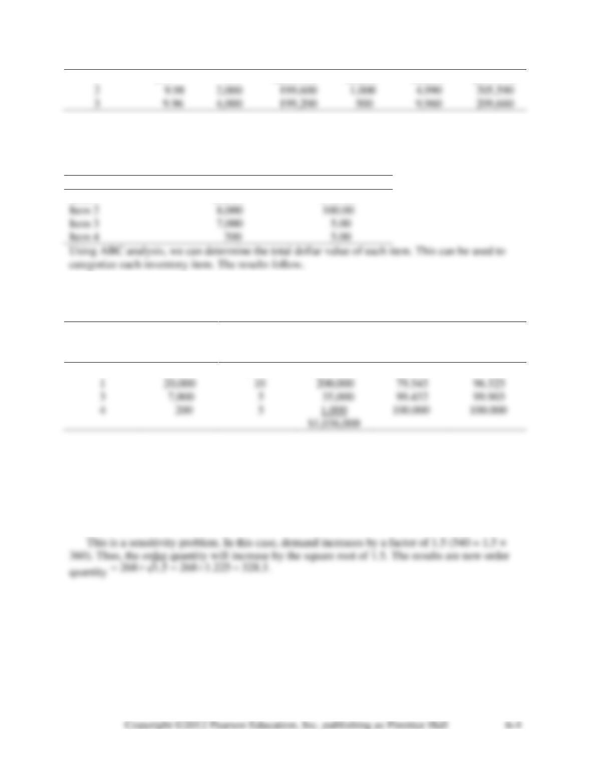
Alternative Example 6.4: Kimberly Caller is in charge of four inventory items. The inventory
demand and sales price for each item is summarized in the following table. Using ABC analysis,
how should these inventory items be controlled?
Demand
Price
Item 1
20,000
$ 10.00
Item 2
100.00
Item 3
As can be seen in the table below, item 2 should be carefully controlled. It is in the A catego-
ry. Item 1 should be controlled to some extent. It is in the B category. Items 3 and 4 should not
be carefully controlled. These items are in the C category.
Cumulative
Cumulative
Item
Annual
Unit
Annual $
Percentage
Percentage
Number
Demand
Cost
Volume
of Items
of Cost
2
8,000
$100
$800,000
22.727
77.220
1
79.545
96.525
3
99.432
99.903
4
200
1,000
Alternative Example 6.6: Fun and Games, Inc. sells a variety of electronic games to children
and adults. Annual demand for super Namco games is 360. Holding cost is $1 per game and or-
dering cost is $100 per order. Fun and Games, Inc., has determined that the economic order
quantity should be 268 units given the foregoing data. What happens to the order quantity if an-
nual demand is underestimated by 50%? In other words, what happens if actual annual demand is
540 units?
SOLUTIONS TO DISCUSSION QUESTIONS AND PROBLEMS
6-1. Inventory is an important consideration for managers because as much as 50% of the total
assets of a company can be tied up in inventory. Because of this large investment in inventory,
6-2. The purpose of inventory control is to regulate the flow of inventory at the various invento-
ry storage locations within the organization. This can be done by determining how much inven-
tory is to be ordered and when the inventory should be ordered.
6-3. Buying inventory can be used as a hedge against inflation. When inflation of inventory
items is high, purchasing inventory at today’s prices can be used as a hedge against future infla-
6-4. Storing large quantities of inventory can eliminate shortages and stockouts. On the other
hand, storing large quantities of inventory can significantly increase the cost of carrying or hold-
6-5. There are a number of assumptions that are made in using the economic order quantity. It is
assumed that the cost of ordering, the cost of holding inventory, and the annual demand are
6-6. Due to the assumptions of the economic order quantity, the necessary costs include the
cost of ordering and the cost of carrying or holding inventory. The cost of the item is included
when ordering costs are a percentage of purchase price.
6-7. The reorder point specifies when an order is to be placed for new inventory items. When the
inventory drops to or below the reorder point, an order is placed.
6-8. The purpose of sensitivity analysis is to determine what effect changes in the annual de-
6-9. The assumptions made in the production run model are the same assumptions made in the
economic order quantity with the exception that the instantaneous receipt of inventory assump-
6-10. When the daily production rate becomes very large, the production run model becomes
identical to the economic quantity model. This is because the fraction d/p approaches zero as the
production rate becomes very large.
6-11. Solving a quantity discount model involves several steps. The first step is to compute the
economic order quantity for each discount range. The second step is to adjust the order quantity
6-12. When the daily demand is normally distributed but the lead time is constant, the standard
deviation of demand during lead time is calculated by multiplying the square root of the lead
time in days by the estimate of the daily standard deviation of demand.
6-13. In using the marginal analysis approach, ML/(ML + MP) is calculated. The probability (P)
of selling the last unit stocked must be at least this great. For discrete distributions, this probabil-
6-14. ABC analysis is the process of categorizing inventory into three groups. The A group is
very costly to the organization and requires strict monitoring and control. The B group is not as
6-15. The overall purpose of MRP is to determine how much to order and when to order items
6-16. The gross material requirements plan does not take into account any existing on-hand in-
ventory. A net material requirements plan uses on-hand inventory to determine the net require-
ments for all items in the structure tree.
6-18. D = 100,000; Co = $10; Ch = $0.005
a.
( )( )
*2 100,000 10 20,000 number 6 screws
0.005
Q==
6-19. ROP = 8 days (500 screws/day) = 4,000 number 6 screws
6-20.
1
2
oh
D
TC C QC
Q
=+
Cost under Lila’s policy
100,000 20, 000
$10 $0.005 $100
20,000 2
= + =
6-21. D = 4,000 units
Ch = 10% of $90 = $9
6-22. Co = $25
Ch = 25% of $100 = $25
6-23. D = 500 sandals; Co = $10
If Q* = 100,
6-24. Optimal order quantity is proportional to the square root of the ordering cost.
When Co = $10, Q* = 20,000 screws
*
If $20, 20,000 2 28, 284 screws
o
CQ= = =
*
If $40, 20,000 4 40, 000 screws
o
CQ= = =
6-25. a.
( )
2 2,500 18.75
2
EOQ 250 units
1.5
o
h
DC
C
= = =
.
b. Average inventory
250 125
22
Q
= = =
6-26. a. daily demand = 2500/250 = 10 units per day
b.
( )
*2 2,500 25
2324.92
10
1.48 1
150
s
h
DC
Qd
Cp
= = =
−
−
Annual holding cost = (average inventory) Ch = 129.97 (1.48) = $192.35
e. Number of production runs = D/Q =2500/324.92 = 7.694
Annual setup cost = (D/Q)Cs = 7.694(25) = $192.35
f. Including the cost of production, the annual cost is
$192.35 + $192.35 + 2,500(14.80) = $37,384.71
g. ROP = d × L = 10 × 0.5 = 5 units
6-27. a. Total cost = ordering cost + holding cost + purchase cost
2
oh
DQ
C C DC
Q
= + +
6-28. During the lead time, the average demand (
) is 2(10) = 20 units per day. The standard de-
viation (
) is 1.5.
6-29.Co = $10; Ch = $10; D = 5,000
( )( )
*2 5,000 10 100 motors
10
Q==
6-30. D = 12,000; Co = $30; Ch = $2
( )( )
*2 12,000 30 600 units
2
Q==
6-31. To begin with, Lisa must determine which costs are not directly related to ordering or car-
rying costs. The cost of new product development, product advertising, and research and devel-
opment are not related to ordering or carrying cost. Lisa must also determine which costs are re-
lated to ordering and carrying costs. See the following table, which was prepared using a spread-
sheet program.
Ordering
Carrying
Cost Factor
Cost
Cost
Taxes
$2,000
Processing and inspec-
tion
$1,500
Bill paying
500
Ordering supplies
Inventory insurance
600
Spoilage
750
Sending purchasing or-
ders
Inventory inquiries
450
Warehouse supplies
280
Purchasing salaries
3,000
Warehouse salaries
2,800
Inventory theft
800
Purchase order supplies
500
Inventory obsolescence
300
$6,800
$7,530
6-32. D = 8,000; d = 40; p = 150; Cs = $100; Ch = $0.30
6-33. D = 10,000; d = 50; p = 500; Co = $40; Ch = $0.60
6-34. D = 1,000; unit cost = $50; Co = $40;
Ch = 0.25 × unit cost
( )( )
( )
2 1,000 40 80
0.25 50
Q==
With discount, unit cost = (1 – 0.03) × $50 = $48.50
6-35.
= 60;
= 7
=
6-36. Ch = $0.50;
= 600;
= 7
Safety stock for 90% service level 9
Carrying cost = 9 × 0.5 = $4.50
6-37. a, b.
Total Cost =
Unit Cost ×
% of
Code
Demand
Total
XX1
$7,008
7
B66
$5,994
6
3CP0
1
33CP
R2D2
$2,220
2
RMS
2
6-38. D = 16,000; Co = $25; i = 0.20
To solve this problem, we must find the economic order quantities and the annual inventory costs
for both Supplier A and Supplier B.

The first order quantity is ignored as the result of 322.75 suggests buying large quantities
at a time. The third order quantity above is infeasible as the price of $34.70 is for purchas-
ing at least 500 and, hence, is adjusted to 500.
Therefore, the preferred quantity for Supplier A is 500. For Supplier B we have:
Similar to Supplier A, the first order quantity is ignored as the result of 318.22 suggests
buying large quantities at a time. The third order quantity above is infeasible as the price
of $34.60 is for purchasing at least 1000 and, hence, is adjusted to 1000.
6-39. D = 5,000; Co = $15; Ch = $0.50; d = 100; t = 3
a.
( )( )
*2 5,000 15 547.7
0.50
Q==
b. The ordering cost is still
o
DC
Q
, but the carrying cost will be reduced because it arrives
over three weeks.
Maximum inventory level = total order – total used during lead time
= Q – 3 × 100
= Q – 300
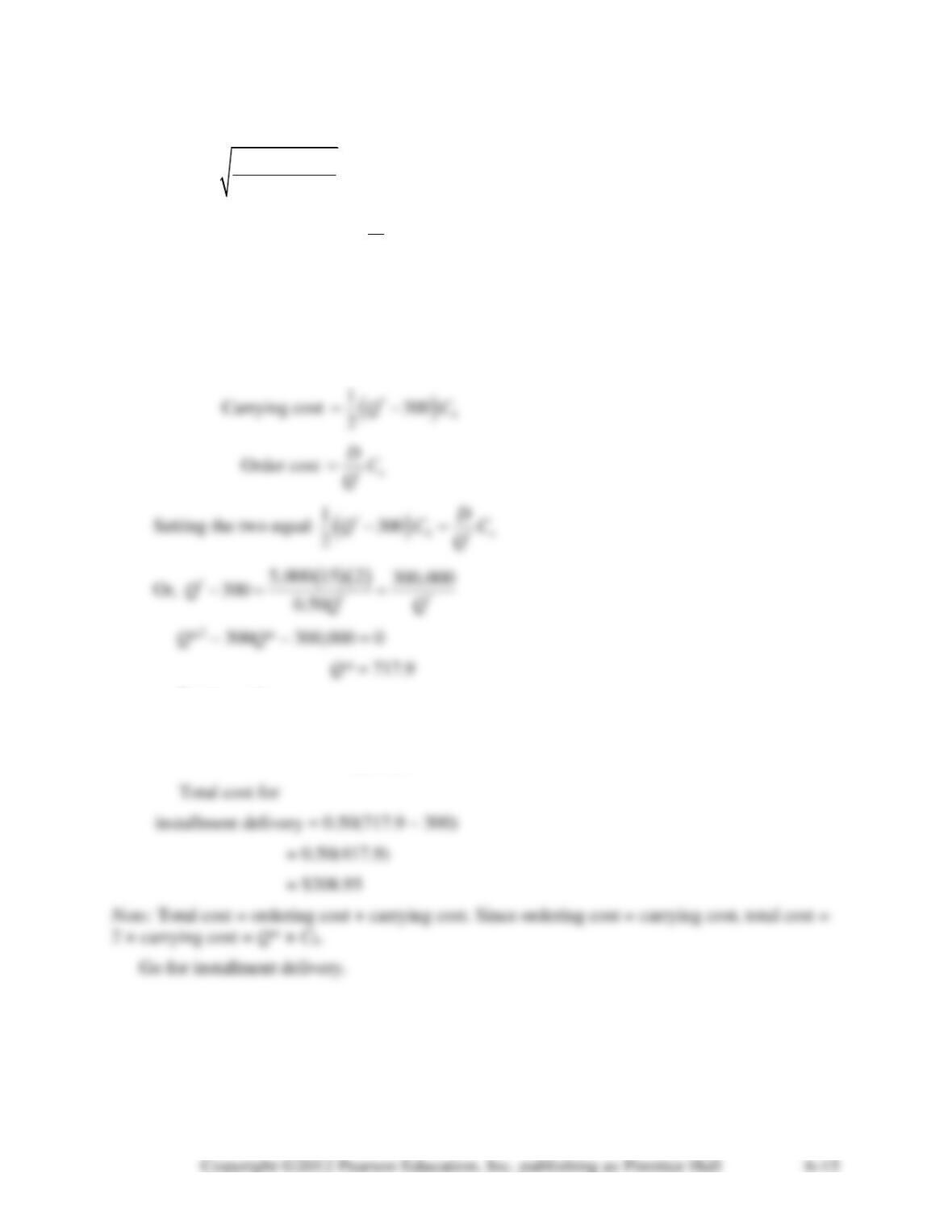
c. Total cost for
instantaneous delivery = 547.7 × 0.50
= $273.85
6-40. Maximum inventory level = Q – 5 × 100
= Q – 500
Carrying cost
( )
1500 0.50
2Q= −
6-41. Demand is constant while lead time is normally distributed:
a. The standard deviation of demand during the lead time is equal to the product of constant
daily demand and the standard deviation of the lead time:
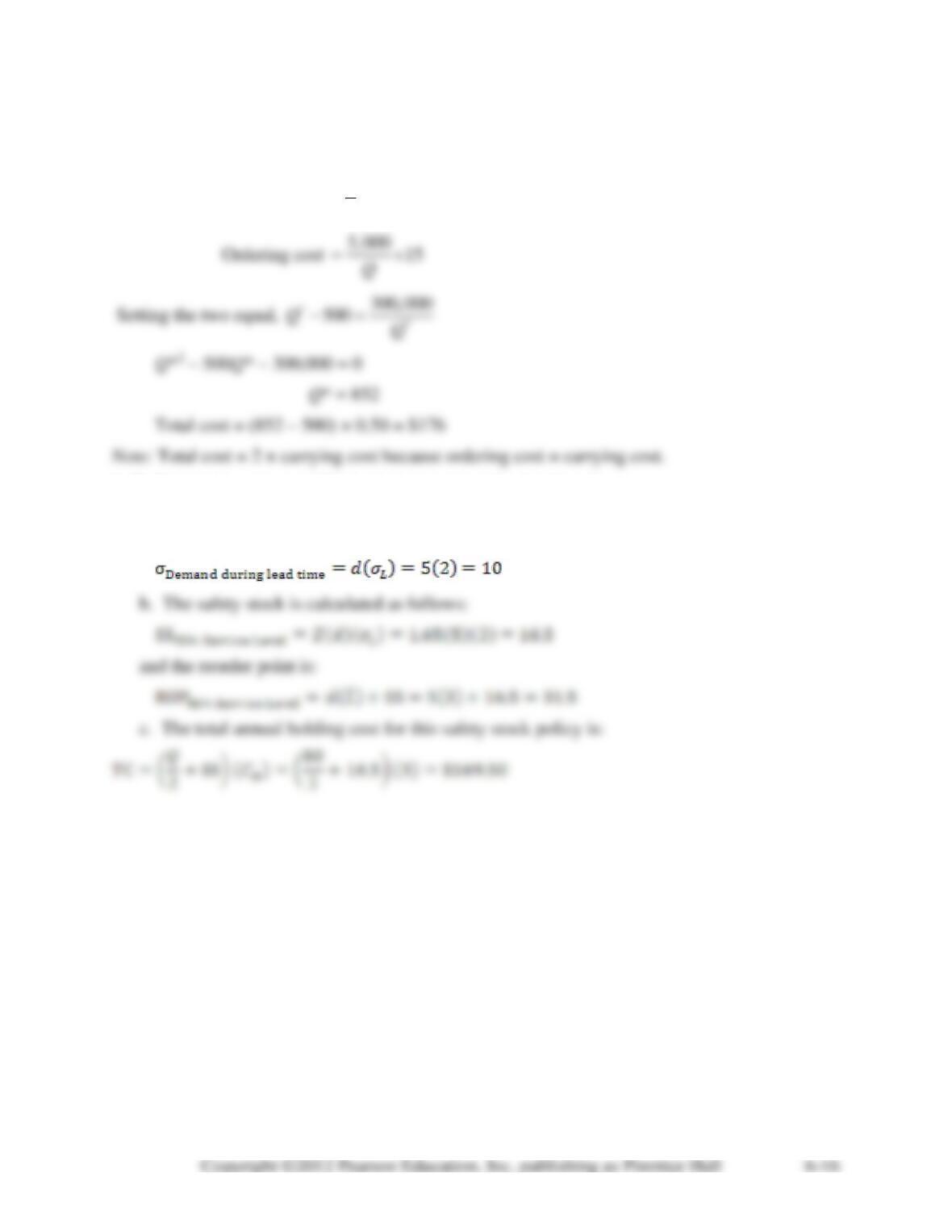
6-42. Lead time is constant while demand is normally distributed:
a. The standard deviation of demand during the lead time is:
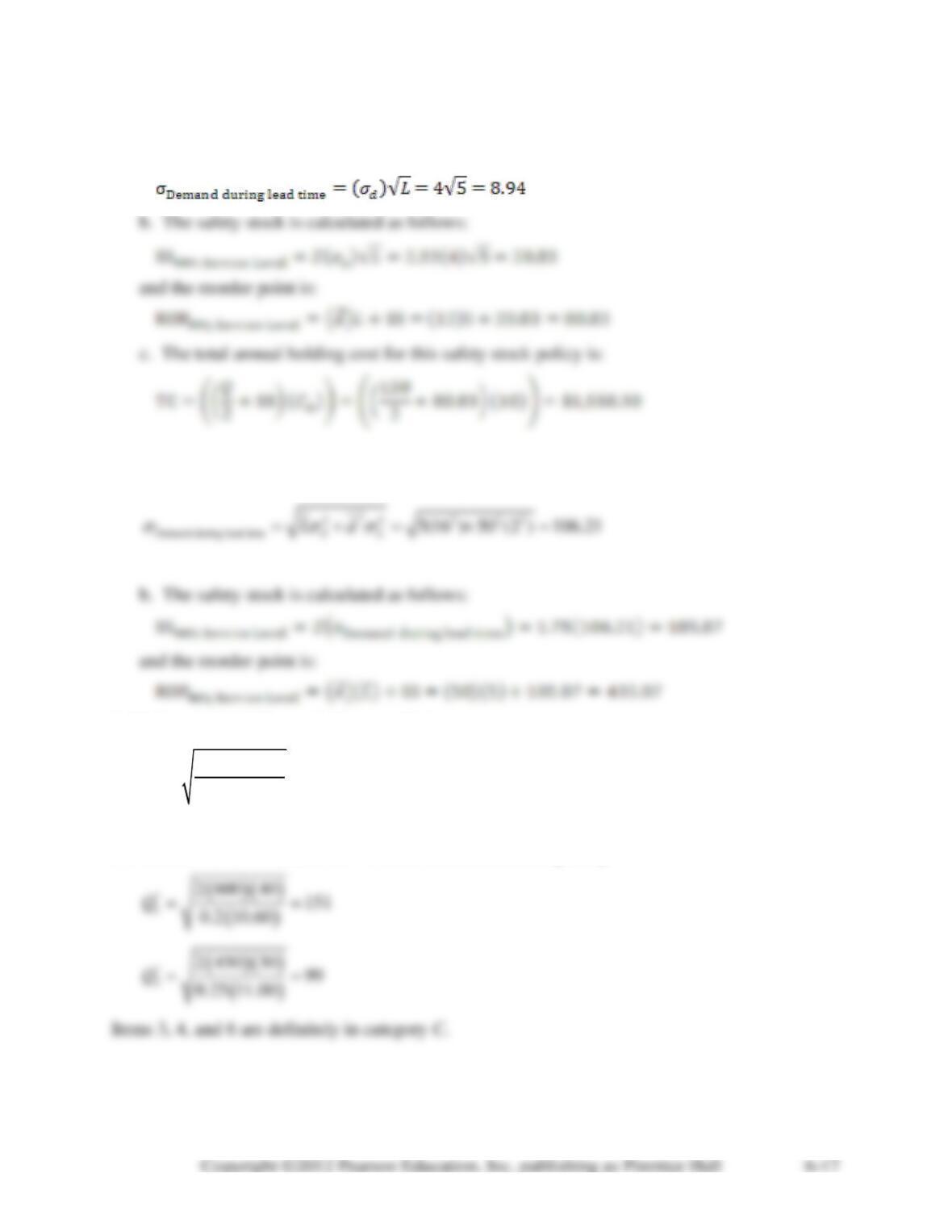
6-43. Both the lead time and the demand are normally distributed:
a. The standard deviation of demand during the lead time is:
6-44. Item 4 should be carefully controlled:
( )( )
( )
*
4
2 560 40 45
0.15 150
Q==
The other items contribute together about 15% of total revenues. They do not need strict quanti-
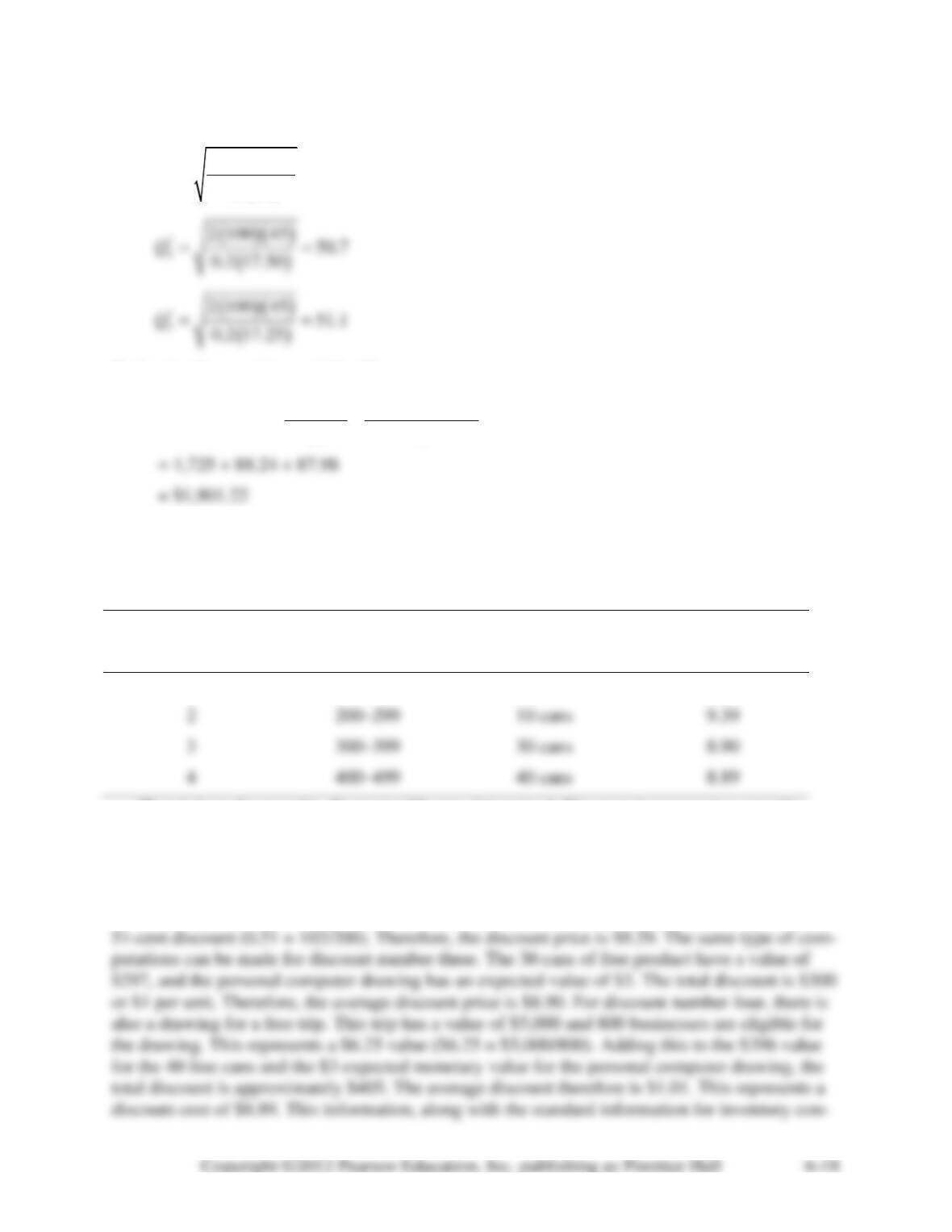
tative control. If however, items 1 and 2 are controlled using EOQ:
*
2
Q==
6-45. Co = $45; I = 20%; D = 100
( )( )
( )
*
1
2 100 45 50
0.2 18
Q==
Optimal order quantity would be 51.
( ) ( ) ( )( )
100 45 51 0.2 17.25
TC 100 17.25 51 2
= + +
6-46. This is a typical quantity discount problem. It is complicated, however, by the fact that
there are drawings for computers and trips, which must be considered as part of the quantity dis-
count. When this is done, a quantity discount table can be developed and used to determine the
best inventory policy. The quantity discount table is shown below.
Average Discount
Discount
Discount
Discount
Discount Cost
1
100–199
0
$9.90
2
200–299
3
300–399
4
400–499
Here is how the quantity discount table was determined. Discount 1 represents a quantity
ranging from 100 to 199 units. There is no discount, and therefore the cost is simply $9.90. For
discount number two, 10 free cans of product are offered. This has a total value of $99. In addi-
tion, it is possible to receive a personal computer valued at $3,000. Since there are 1,000 compa-
nies that are eligible, the expected monetary value for the personal computer drawing is $3 (3 =
3,000/1,000). This represents a total discount of $102. For 200 cans of product, this represents a
6-47. a. This is a typical quantity discount problem. The data and results are presented below.
The optimal quantity is 1,500 disks.
Data
Demand rate (D)
2,000
Setup/Ordering cost (S)
250
Holding rate (I)
10%
Price Ranges
From
To
Price
1
500
$10
Results
Optimal order quantity (Q*)
1,501.
Average inventory
750.
Production runs per period (year)
1.33
Annual Setup cost
Annual Holding cost
Unit costs (PD)
Total Cost (rounded)
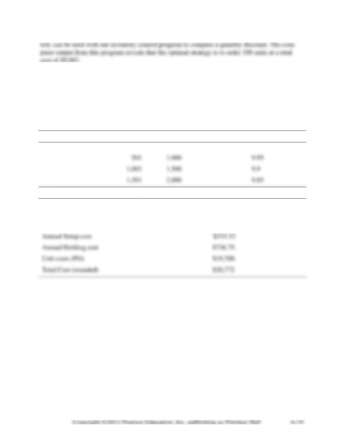
6-47. b. Given a different quantity discount schedule, we can compute the optimal order policy
using the same approach. The results are shown below.
Data
Demand rate (D)
2,000
Setup/Ordering cost (S)
$250
Holding rate (I)
10%
Price Ranges
From
To
Price
1
500
$10
501
1,000
9.99
1,001
1,500
9.98
1,501
2,000
9.97
Results
Optimal order quantity (Q*)
1,001
Average inventory
500.50
Production runs per period (year)
2
Annual Setup cost
Annual Holding cost
Total Cost
$20,960.00
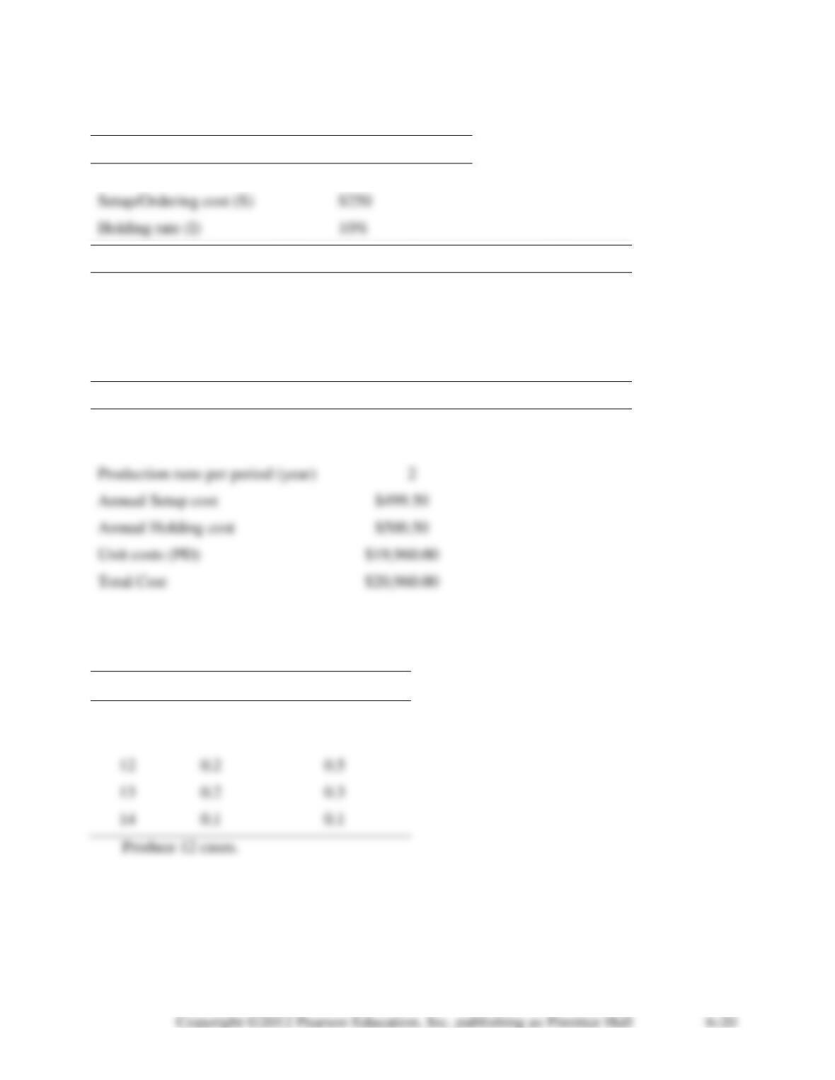
6-48. ML = 75 – 50 = 25; MP = 100 – 75 = 25
ML/(ML + MP) = 25/(25 + 25) = 0.5
Demand
Probability
P(Demand _____)
10
0.2
1.0
11
0.3
0.8
12
0.2
0.5
14
0.1
0.1