49
CHAPTER 6: INVENTORY ANALYSIS
6.1 Objective
This chapter is the first on inventory. We use it as an introduction to “supply chain management”
6.2 Additional Suggested Readings
We assign a short case as supplemental reading for the economies of scale. The case is used to show
Suggested assignment questions:
1. What factors should be taken into consideration when deciding the batch size of a particular type of
printer shipped to Europe (or any other destination)? What do you think of the fact that “inventory
6.3 Solutions to the Problem Set
Problem 6.1
The data in the question is: flow rate R = 50,000 parts/yr, fixed ordering cost S = $800, purchasing cost C
= $4/part, and cost of capital r = 20%/yr. Thus, the annual unit holding cost is H = rC = $0.8/yr. The
Problem 6.2
BIM Computers: Assume 8 working hours per day.
Chapter 6
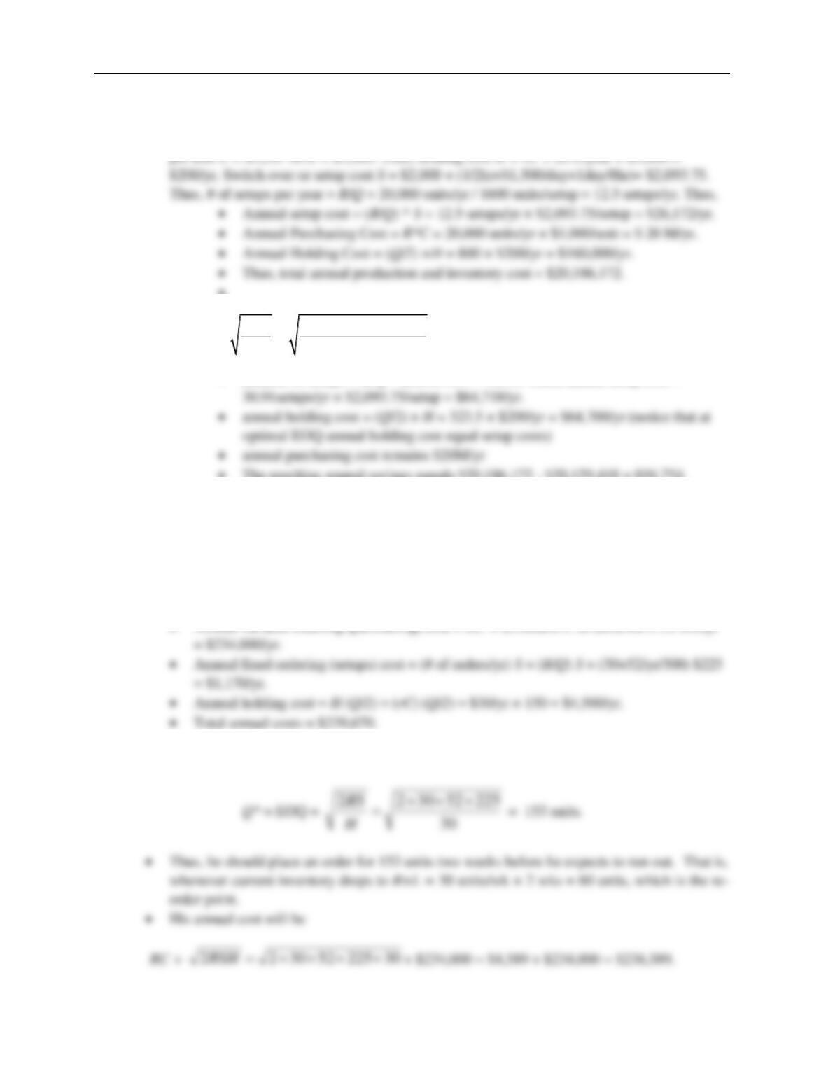
• We know Q = 4 wks supply = 1,600 units; R = 400 units/wk = 20,000 units/yr; purchase cost
•
• EOQ =
2 2 20000 2093.75
200
RS
H
=
= 647 units.
• number of setups = R/Q = 20,000 /647 = 30.91. Thus, annual setup cost =
• The resulting annual savings equals $20,186,172 – $20,129,418 = $56,754.
Problem 6.3
Victor’s data: flow unit = one dress, flow rate R = 30 units/wk, purchase cost C = $150/unit, order lead
time L = 2 weeks, fixed order cost S = $225, cost of capital r = 20%/yr. Victor currently orders ten weeks
supply at a time, hence Q = 10wks × 30 units/wk = 300 units.
a. Costs for Victor’s current inventory management:
• Annual variable ordering (purchasing) cost = RC = $150/unit × 30 units/wk × 52 wks/yr
b. To minimize costs, Victor should order in batches of
Chapter 6
Problem 6.4
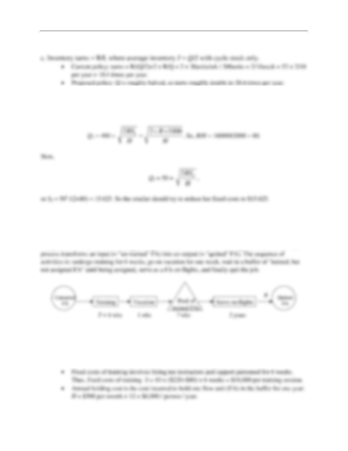
The retailer: Current fixed costs, S1 = $1000. Current optimal lot size Q1 = 400. New, desired lot size Q2
= 50. We must find the fixed cost S2 at which Q2 is optimal. Since Q1 is optimal for S1, we have
Problem 6.5
Major Airlines: This question illustrates the basic tradeoff between fixed and variable costs in a service
industry; thus the concepts of EOQ discussed in class in the context of inventory management are much
more generic.
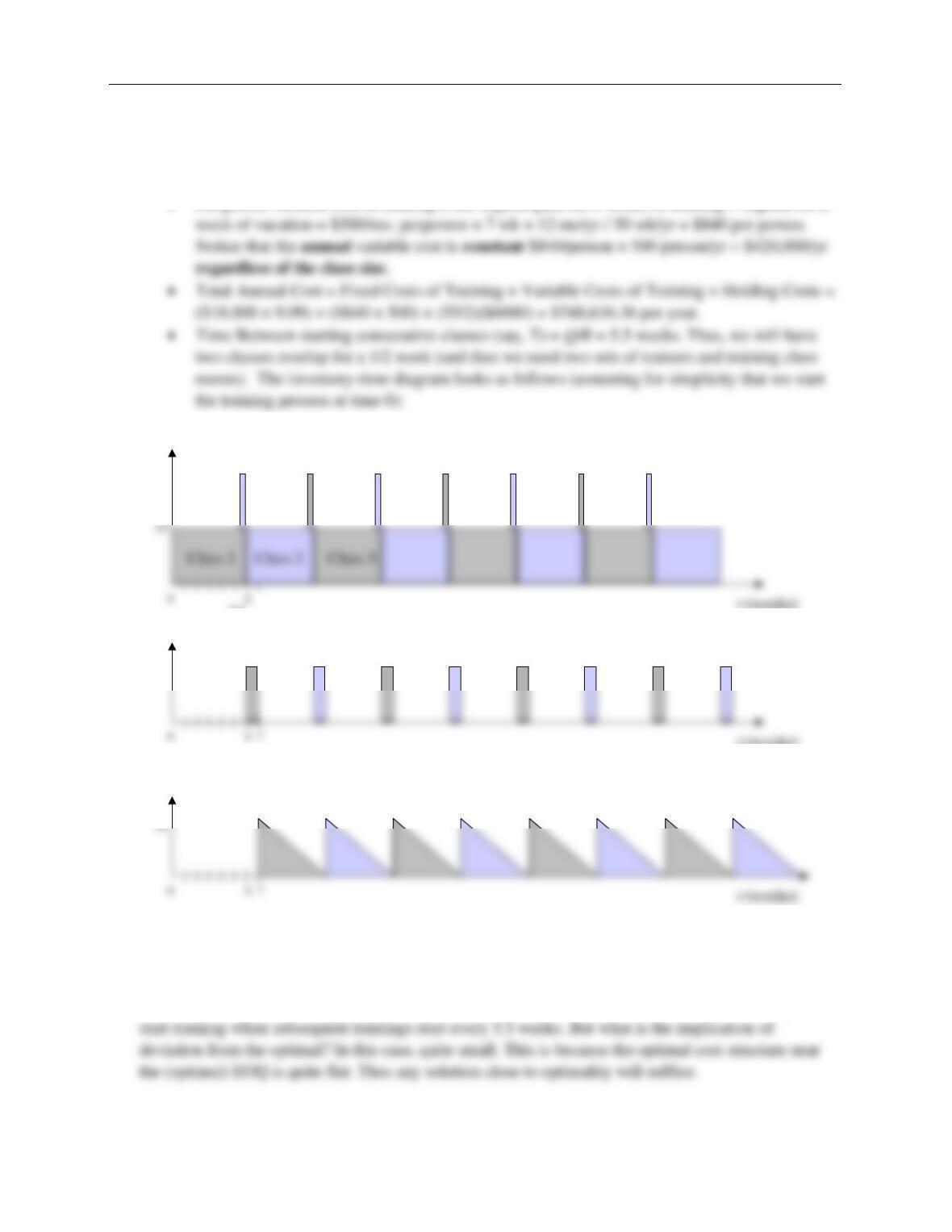
The process view here is illuminating and it goes as follows: flow unit = one flight attendant (FA). The
The question asks for the tradeoff between training costs (higher class size is preferred) versus ‘holding
costs’ in the buffer (smaller class size -> fewer attendants waiting in buffer is preferred).
• (a)
• Flow rate R = 1000 every two years = 500 attendants per year = 10 per week.
Chapter 6
• Thus, Economic Class Size (EOQ) = 54.77 or 55 per class. Thus, we should run R/Q = 500 /
55 = 9.09 classes per year
• Per person variable cost of training is the stipend paid for 6 weeks of training + stipend for a
t (weeks)
I (in training)
5.56
110
t (weeks)
I (on vacation)
55
I (in buffer)
Class 1 Class 2 Class 3
Class 1 Class 2 Class 3
• (b): This part of the question illustrates the following: Often, in reality, people wish to adopt policies
that are simple (e.g., starting training every 6 weeks is simpler than trying to track the exact days to
Chapter 6
Problem 6.6
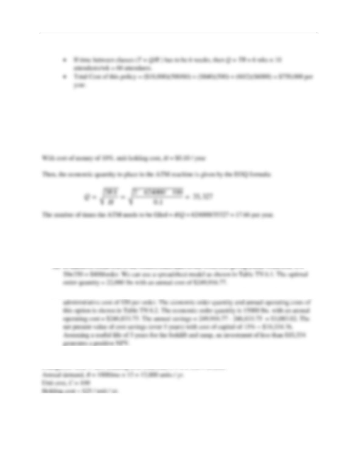
Fixed cost of filling an ATM m/c, S = $100.
To estimate demand, observe that the average size of each transaction = $80. With 150 transactions per
week, annual demand R is estimated to be = 150×52×80 = 624,000.
Problem 6.7
The annual demand, R = 150,000 lbs/yr. The purchase price per lb is $1.50. However the shipping cost
exhibits a quantity discount model. The holding cost per year is then 15% of the sum of the purchase and
shipping cost. The administrative costs of placing an order = $50/order.
(b) If GC buys a forklift and builds a new ramp, then the per-transaction fixed cost will simply be the
Problem 6.8
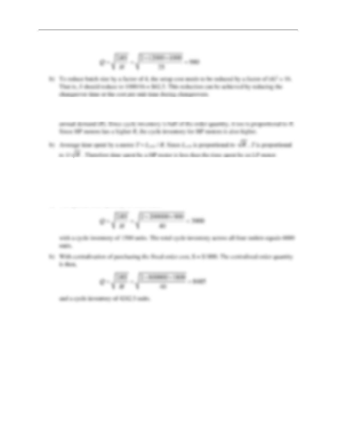
a) The optimal production batch size is
Chapter 6
Problem 6.9
a) From the EOQ formula, observe that the order quantity is proportional to the square root of
Problem 6.10
Each retail outlet faces an annual demand, R = 4000/wk × 50 = 200,000 per year. The unit cost of the
item, C = $200 / unit. The fixed order cost, S = $900. The unit holding cost per year, H = 20 % × 200 =
$40 / unit / year.
a) The optimal order quantity for each outlet