
Excel Templates to accompany Operations Management, Eleventh Edition
created by Lee Tangedahl
Copyright © 2012 by The McGraw Hill Companies, Inc. All rights reserved.
Supplement to Chapter Five – Decision Theory
Templates: Payoff Table (B) Solved Problems: Solved Problem 1,3,4a
Decision Tree Solved Problem 4b
Sensitivity Analysis Solved Problem 2
Lecture Suggestions Problems 8-12
Example 5
Example 8
See Instructions template for complete instructions.
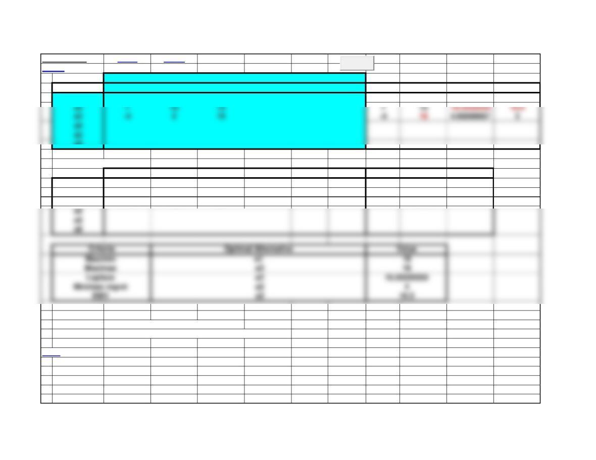
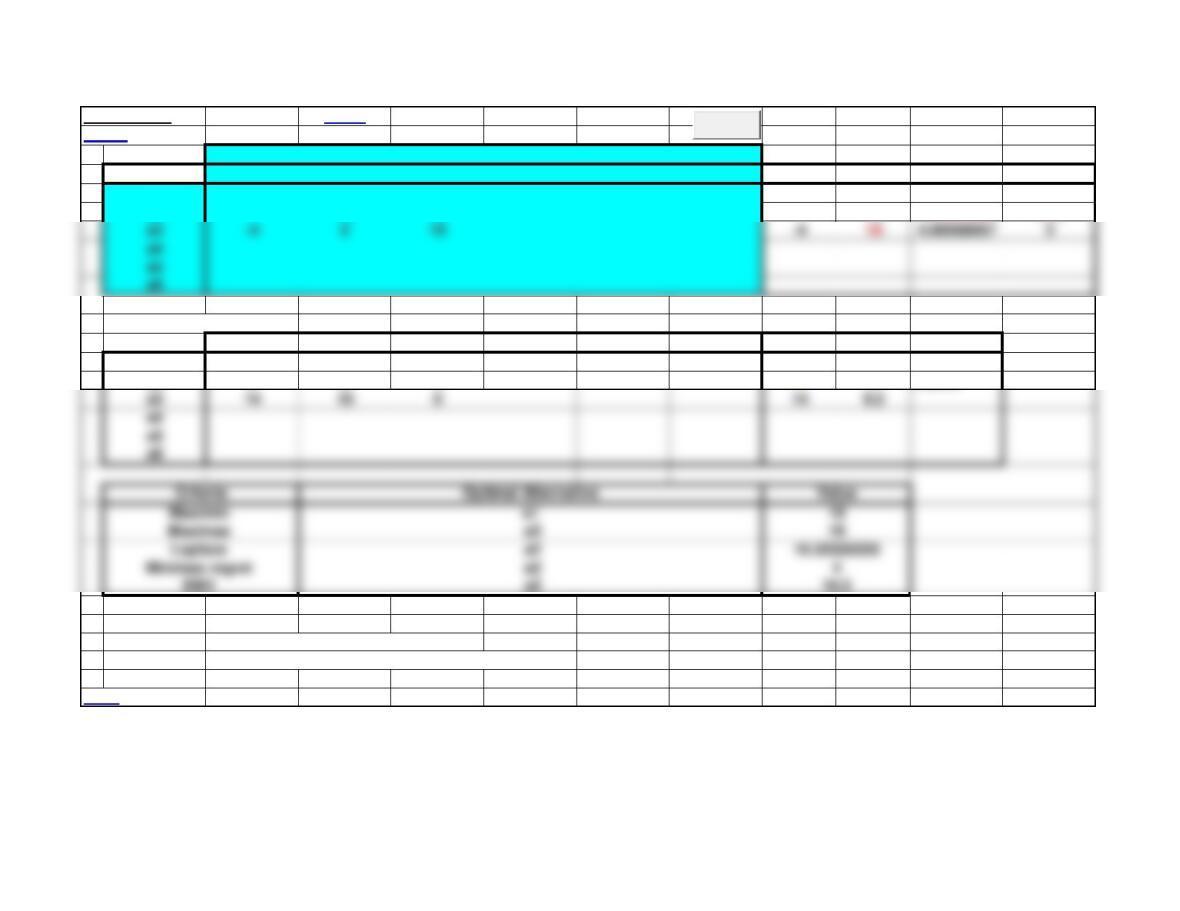
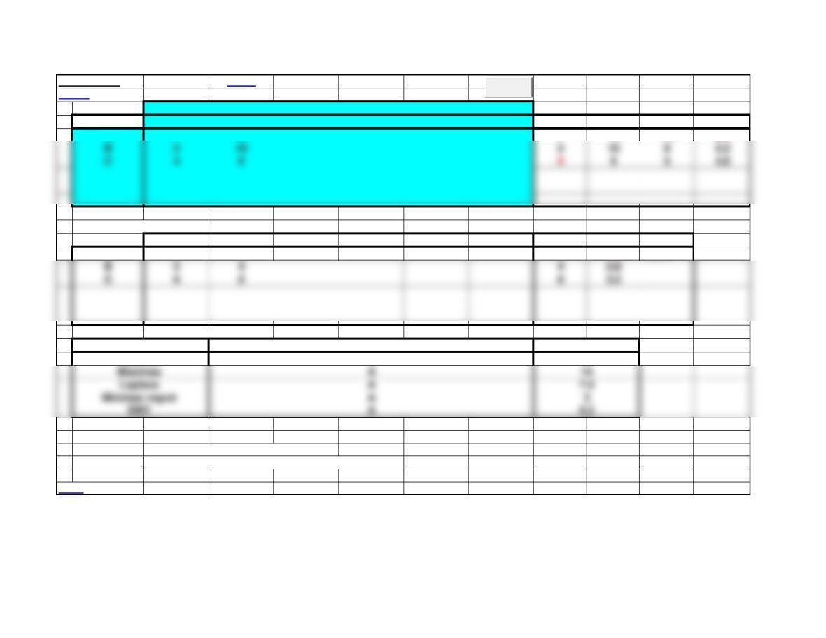
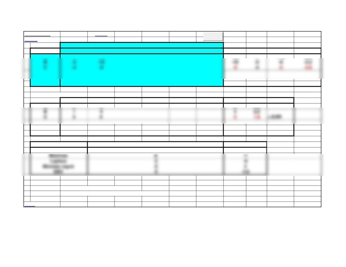
Payoff Table
Payoff Table Basic Notes
<Back
s1 s2 s3 s4 s5 s6 SProb = 1
Probability = 0.3 0.5 0.2 Min Max Avg EMV
a1 10 10 10 10 10 10 10
a6
Opportunity Loss Table
s1 s2 s3 s4 s5 s6 Max EOL
a1 0 2 6 6 2.2
a2 3 0 4 41.7 = EVPI
a3 14 10 014 9.2
a4
a5
a6
Notes: Enter costs as negative numbers.
Be sure unused cells are blank (deleted), NOT zero.
^Top
Clear
Page 2
a2 712 12 712 10.3333333 10.5
a4
a5
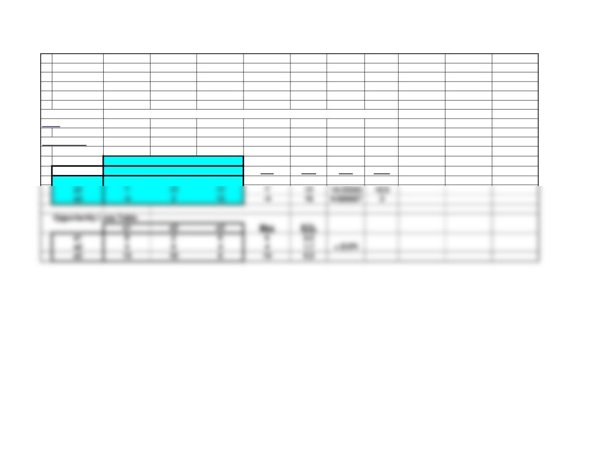
Payoff Table
Basic Template: You can simply copy the basic template below and paste into another worksheet.
^Top
Payoff Table
s1 s2 s3 SProb = 1
Probability = 0.3 0.5 0.2 Min Max Avg EMV
a1 10 10 10 10 10 10 10
Page 3
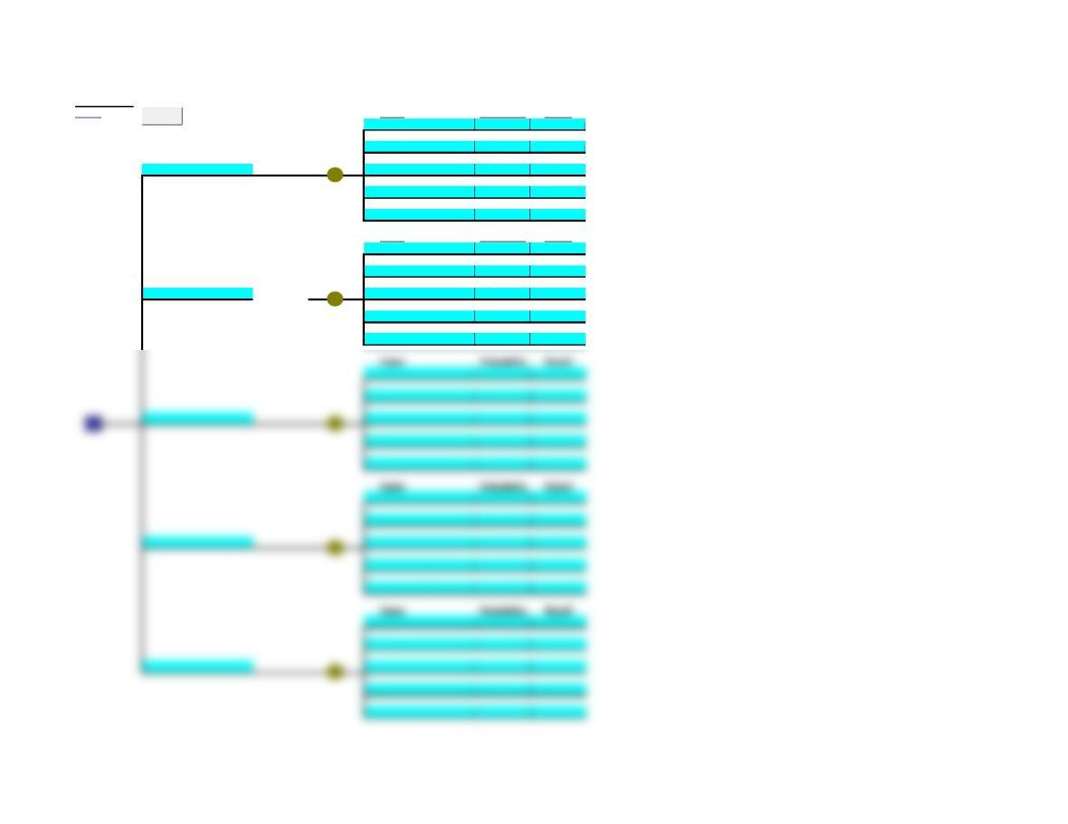
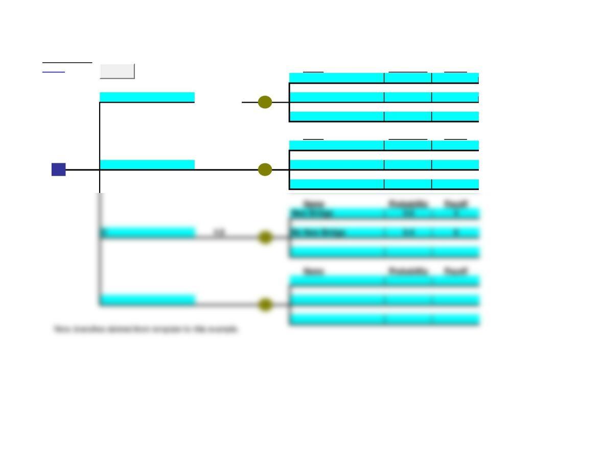
Decision Tree
<Back Name Probability Payoff
0.4 40
0.6 55
Build Small 49
Name Probability Payoff
0.4 50
0.6 70
Build Large 62
Low Demand
High Demand
Low Demand
High Demand
Clear
Name Probability Payoff
Name Probability Payoff
Name Probability Payoff
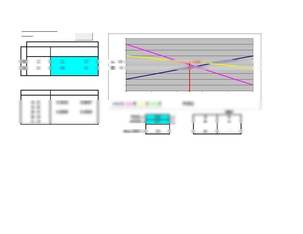
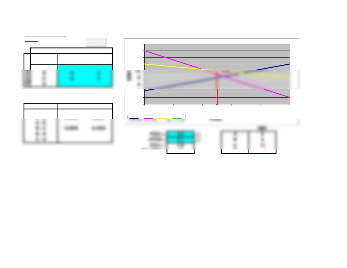
Sensitivity Analysis
<Back
P(S2) A B C D
Payoff Table TRUE TRUE TRUE FALSE
States of Nature 0.000 4.00 16.00 12.00 #N/A
S1 S2 0.100 4.80 14.60 11.60 #N/A
B16 20.300 6.40 11.80 10.80 #N/A
C12 80.400 7.20 10.40 10.40 #N/A
D0.500 8.00 9.00 10.00 #N/A
0.600 8.80 7.60 9.60 #N/A
0.700 9.60 6.20 9.20 #N/A
0.800 10.40 4.80 8.80 #N/A
Intersection P(S1) P(S2) 0.900 11.20 3.40 8.40 #N/A
A – B 0.4545 0.5455 1.000 12.00 2.00 8.00 #N/A
A – C 0.3333 0.6667 0.500 0.00
A – D 0.500 10.00
P(S1) = 0.5 C10
Alternative
0
2
4
6
12
14
16
18
0.000 0.200 0.400 0.600 0.800 1.000
EMV
Clear
Lecture Suggestions – Supplement to Chapter 5
<Back
Example 8: Sensitivity Analysis
1. Select the Example 8 worksheet, note that the payoffs for each alternative (A, B, C) under both
states of nature (S1, S2) have been entered.
2. Point out in the EMV graph that the EMV for each alternative have been graphed as a line for values
of the probability of S2 between 0 and 1. For example, the EMV for alternative A is graphed in the dark
4. Now determine which alternative has the maximum EMV for different values of P(S2).
a. Start with P(S2) = 0 and point out that alternate B has the maximum EMV=16, as shown in red
in the same table in the lower right
c. Continue to click the spinner button and point out that when P(S2) is between .4 and .6,
5. Finally, determine the exact range of optimality for each alternative. The table in the lower left
hand corner shows the intersection for the lines B and C is at P(S2)=.4 and the intersection for lines A
Example 2,3,4,7
Payoff Table Notes
<Back
s1 s2 s3 s4 s5 s6 SProb = 1
Probability = 0.3 0.5 0.2 Min Max Avg EMV
a1 10 10 10 10 10 10 10
a2 712 12 712 10.3333333 10.5
Opportunity Loss Table
s1 s2 s3 s4 s5 s6 Max EOL
a1 0 2 6 6 2.2
a2 3 0 4 41.7 = EVPI
a3 14 10 014 9.2
a4
a5
Notes: Enter costs as negative numbers.
Be sure unused cells are blank (deleted), NOT zero.
^Top
Clear
Page 7
a4
a5
Decision Tree
<Back Name Probability Payoff
0.4 40
Build Small 49 0.6 55
Name Probability Payoff
Low Demand
High Demand
Clear
0.4 50
Build Large 62 0.6 70
Name Probability Payoff
Name Probability Payoff
Low Demand
High Demand
Sensitivity Analysis
<Back
P(S2) A B C D
Payoff Table TRUE TRUE TRUE FALSE
States of Nature 0.000 4.00 16.00 12.00 #N/A
S1 S2 0.100 4.80 14.60 11.60 #N/A
A 4 12 0.200 5.60 13.20 11.20 #N/A
0.600 8.80 7.60 9.60 #N/A
0.700 9.60 6.20 9.20 #N/A
0.800 10.40 4.80 8.80 #N/A
Intersection P(S1) P(S2) 0.900 11.20 3.40 8.40 #N/A
A – B 0.4545 0.5455 1.000 12.00 2.00 8.00 #N/A
A – C 0.3333 0.6667 0.500 0.00
A – D 0.500 10.00
Max EMV = 10 D
0
2
4
12
14
16
18
0.000 0.200 0.400 0.600 0.800 1.000
Clear
Solved Problem 1, 3, 4a
Payoff Table Notes
<Back
New Bridge No SProb = 1
Probability = 0.6 0.4 Min Max Avg EMV
A 1 14 114 7.5 6.2
Opportunity Loss Table
New Bridge No Max EOL
A 3 0 31.8 = EVPI
Criteria Optimal Alternative Value
Maximin C 4
Notes: Enter costs as negative numbers.
Be sure unused cells are blank (deleted), NOT zero.
^Top
Clear
Page 10
C 4 6 46 5 4.8
Sensitivity Analysis
<Back
P(S2) A B C D
Payoff Table TRUE TRUE TRUE FALSE
States of Nature 0.000 1.00 2.00 4.00 #N/A
S1 S2 0.100 2.30 2.80 4.20 #N/A
A 1 14 0.200 3.60 3.60 4.40 #N/A
0.600 8.80 6.80 5.20 #N/A
0.700 10.10 7.60 5.40 #N/A
0.800 11.40 8.40 5.60 #N/A
Intersection P(S1) P(S2) 0.900 12.70 9.20 5.80 #N/A
A – B 0.8000 0.2000 1.000 14.00 10.00 6.00 #N/A
A – C 0.7273 0.2727 0.500 0.00
A – D 0.500 7.50
P(S1) = 0.5 C 5
Max EMV = 7.5 D
0
2
4
10
12
14
16
0.000 0.200 0.400 0.600 0.800 1.000
Clear
Decision Tree
<Back Name Probability Payoff
0.6 1
A6.2 0.4 14
Name Probability Payoff
0.6 2
B5.2 0.4 10
No New Bridge
New Bridge
No New Bridge
New Bridge
Clear
Name Probability Payoff
0.6 4
C4.8 0.4 6
Name Probability Payoff
No New Bridge
New Bridge
Solved Problem 6
Payoff Table Notes
<Back
New Bridge No SProb = 1
Probability = 0.6 0.4 Min Max Avg EMV
A-1 -14 -14 -1 -7.5 -6.2
Opportunity Loss Table
New Bridge No Max EOL
Criteria Optimal Alternative Value
Maximin C -6
Notes: Enter costs as negative numbers.
Be sure unused cells are blank (deleted), NOT zero.
^Top
Clear
Page 13