CHAPTER 5
Forecasting
TEACHING SUGGESTIONS
Teaching Suggestion 5.1: Wide Use of Forecasting.
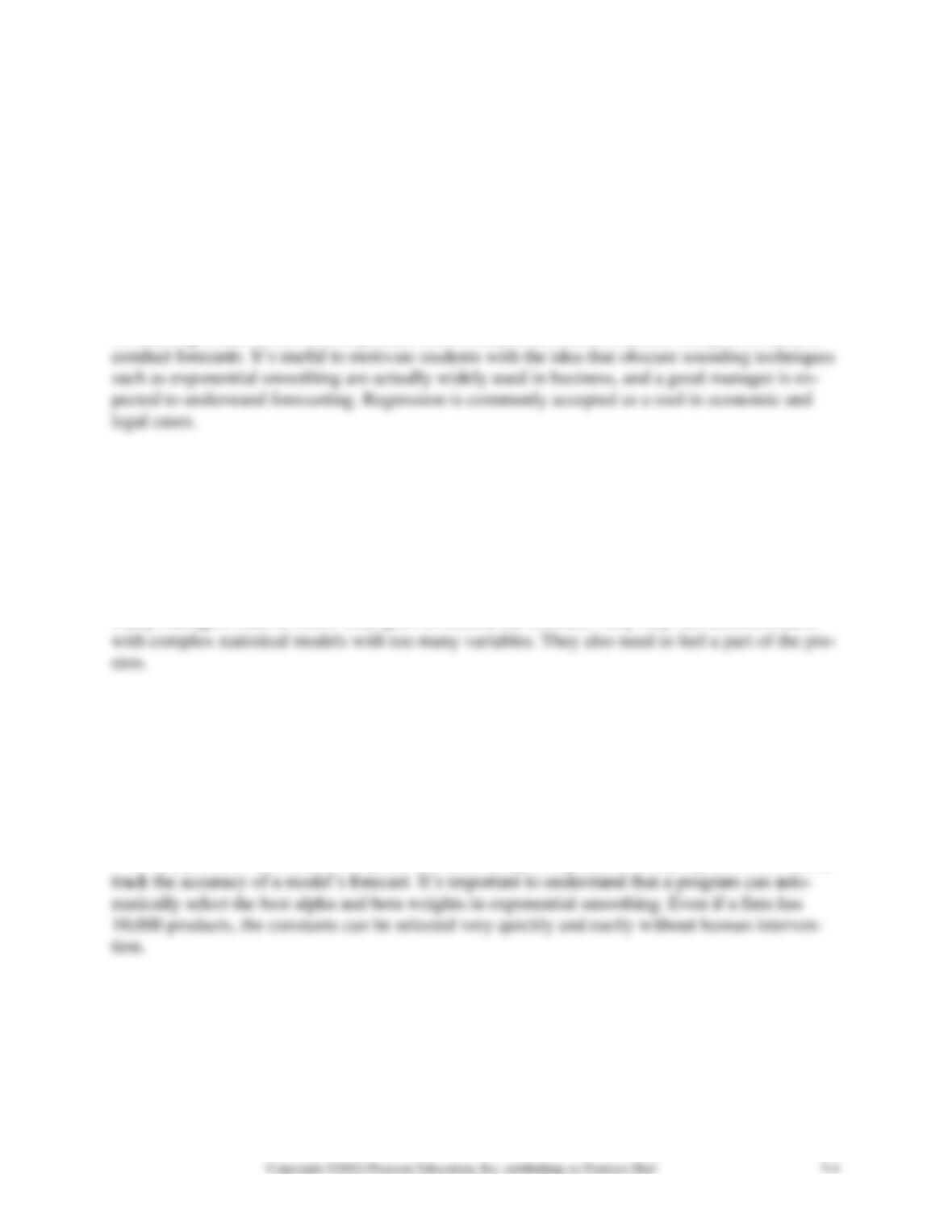
Forecasting is one of the most important tools a student can master because every firm needs to
Teaching Suggestion 5.2: Forecasting as an Art and a Science.
Forecasting is as much an art as a science. Students should understand that qualitative analysis
(judgmental modeling) plays an important role in predicting the future since not every factor can
be quantified. Sometimes the best forecast is done by seat-of-the-pants methods.
Teaching Suggestion 5.3: Use of Simple Models.
Many managers want to know what goes on behind the forecast. They may feel uncomfortable
Teaching Suggestion 5.4: Management Input to the Exponential Smoothing Model.
One of the strengths of exponential smoothing is that it allows decision makers to input constants
that give weight to recent data. Most managers want to feel a part of the modeling process and
appreciate the opportunity to provide input.
Teaching Suggestion 5.5: Wide Use of Adaptive Models.
With today’s dominant use of computers in forecasting, it is possible for a program to constantly
ALTERNATIVE EXAMPLES
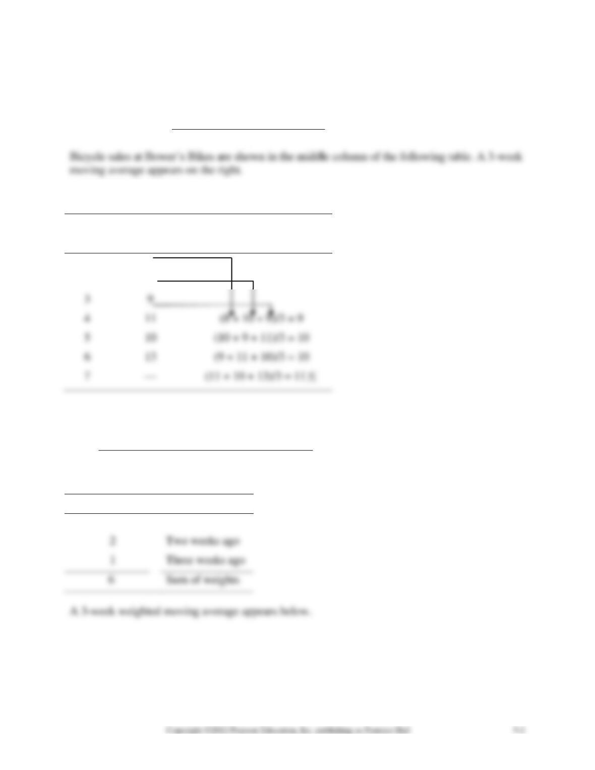
Alternative Example 5.1:
Moving average
demand in previous periodsn
n
=
[ADD ARROWS TO BELOW TABLE]
Actual
Three-Week
Week
Bicycle Sales
Moving Average
1
8
2
10
3
9
4
11
5
10
6
13
Alternative Example 5.2: Weighted moving average
( )( )
weight for period demand in period
weights
nn
=
Bower’s Bikes decides to forecast bicycle sales by weighting the past 3 weeks as follows:
Weights Applied
Period
3
Last week
2
Two weeks ago
6
Sum of weights
Week
Actual Bicycle Sales
Three-Week Moving Average
1
8
–
2
10
–
3
9
–
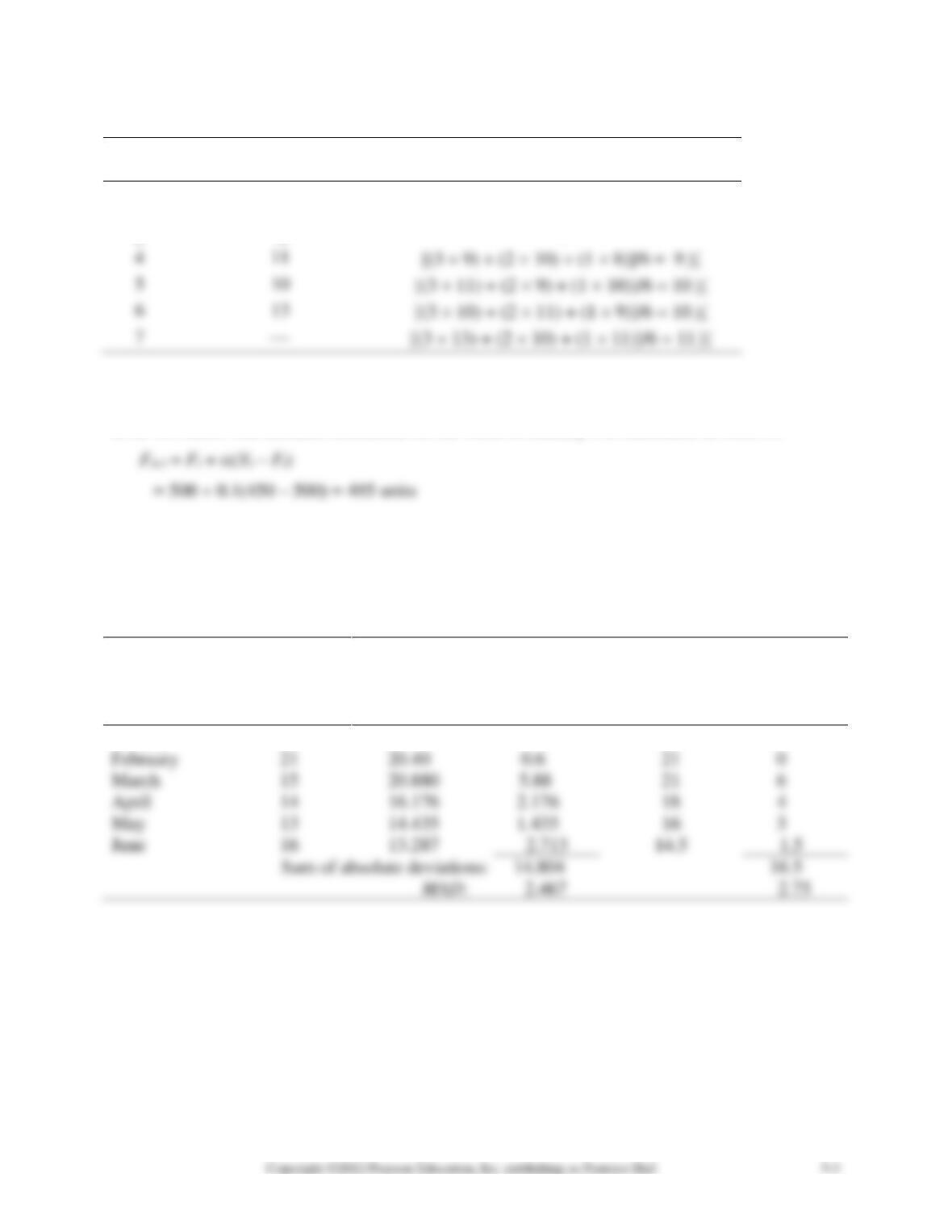
Alternative Example 5.3: A firm uses simple exponential smoothing with
= 0.1 to forecast
demand. The forecast for the week of January 1 was 500 units, whereas actual demand turned out
to be 450 units. The demand forecasted for the week of January 8 is calculated as follows.
Alternative Example 5.4: Exponential smoothing is used to forecast automobile battery sales.
Two values of are examined, = 0.8 and = 0.5. To evaluate the accuracy of each smoothing
constant, we can compute the absolute deviations and MADs. Assume that the forecast for Janu-
ary was 22 batteries.
Absolute
Absolute
Actual
Forecast
Deviation
Forecast
Deviation
Battery
with
With
with
with
Month
Sales
= 0.8
= 0.8
= 0.5
= 0.5
January
20
22
2
22
2
February
21
21
0
March
15
21
6
April
14
18
4
May
13
16
3
June
16
2.713
Sum of absolute deviations: 14.804 16.5
On the basis of this analysis, a smoothing constant of = 0.8 is preferred to = 0.5 because it
has a smaller MAD.
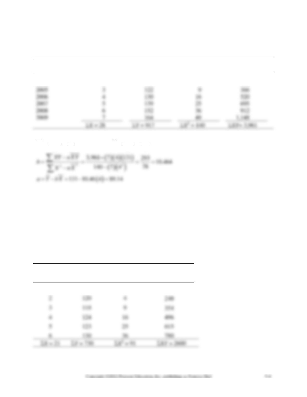
Alternative Example 5.5: Use the sales data given below to determine: (a) the least squares
trend line, (b) the predicted value for 2010 sales.
Time
Sales
Year
Period
(Units)
X2
XY
2003
1
100
1
100
2004
2
110
4
220
2005
3
122
9
366
2006
4
130
520
2007
5
139
695
2008
6
152
912
2009
7
164
28 917
4 131
77
XY
XY
nn
= = = = = =
The trend equation is
^
01 89.14 10.464Y b b X X= + = +
To project demand in 2010, we denote the year 2010 as x = 8,
Sales in 2000 = 89.14 + 10.464(8) = 172.85
Alternative Example 5.6: The rated power capacity (in hours/ week) over the past 6 years is
shown in the table below.
Capacity
Year
(Y)
X2
XY
1
115
1
2
120
4
3
118
9
124
130
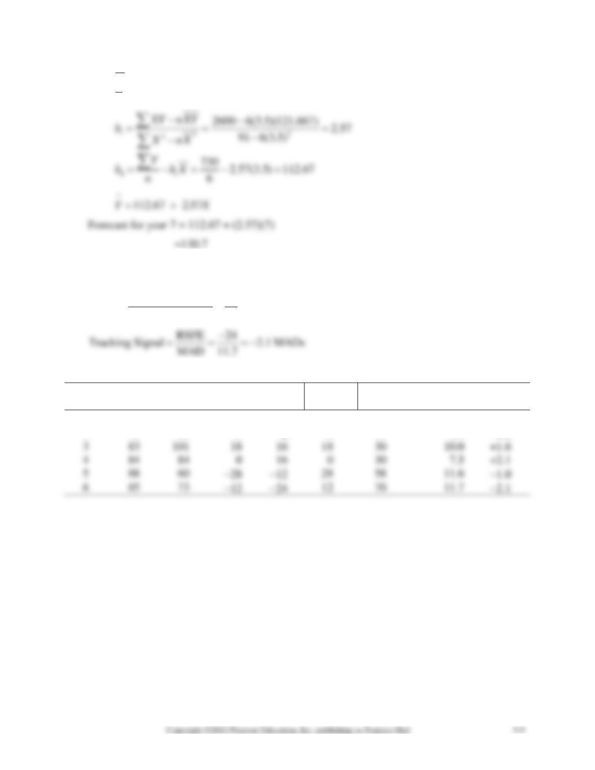
21/ 6 3.5
730 / 6 121.667
X
Y
==
==
Alternative Example 5.7: The forecast demand and actual demand for 10-foot fishing boats are
shown below. We compute the tracking signal and MAD.
Forecast errors 70
MAD 11.7
6n
= = =
Table for Alternate Example 5.7
Forecast
Actual
Forecast
Cumulative
Tracking
Year
Demand
Demand
Error
RSFE
Error
Error
MAD
Signal
1
78
71
−7
−7
7
7
7.0
−1.0
2
75
80
5
−2
5
12
6.0
−0.3
5
88
60
28
58
11.6
−1.0
6
85
73
12
70
11.7
−2.1
SOLUTIONS TO DISCUSSION QUESTIONS AND PROBLEMS
5-1. The steps that are used to develop any forecasting system are:
1. Determine the use of the forecast.
3. Determine the time horizon of the forecast.
5. Gather the necessary data.
7. Make the forecast.
5-2. A time-series forecasting model uses historical data to predict future trends.
5-3. The only difference between causal models and time-series models is that causal models
take into account any factors that may influence the quantity being forecasted. Causal models use
historical data as well. Time-series models use only historical data.
5-4. Qualitative models incorporate subjective factors into the forecasting model. Judgmental
5-6. When the smoothing value, , is high, more weight is given to recent data. When is low,
more weight is given to past data.
5-7. The Delphi technique involves analyzing the predictions that a group of experts have made,
5-8. MAD is a technique for determining the accuracy of a forecasting model by taking the av-
5-9. The number of seasons depends on the number of time periods that occur before a pattern
repeats itself. For example, monthly data would have 12 seasons because there are 12 months in
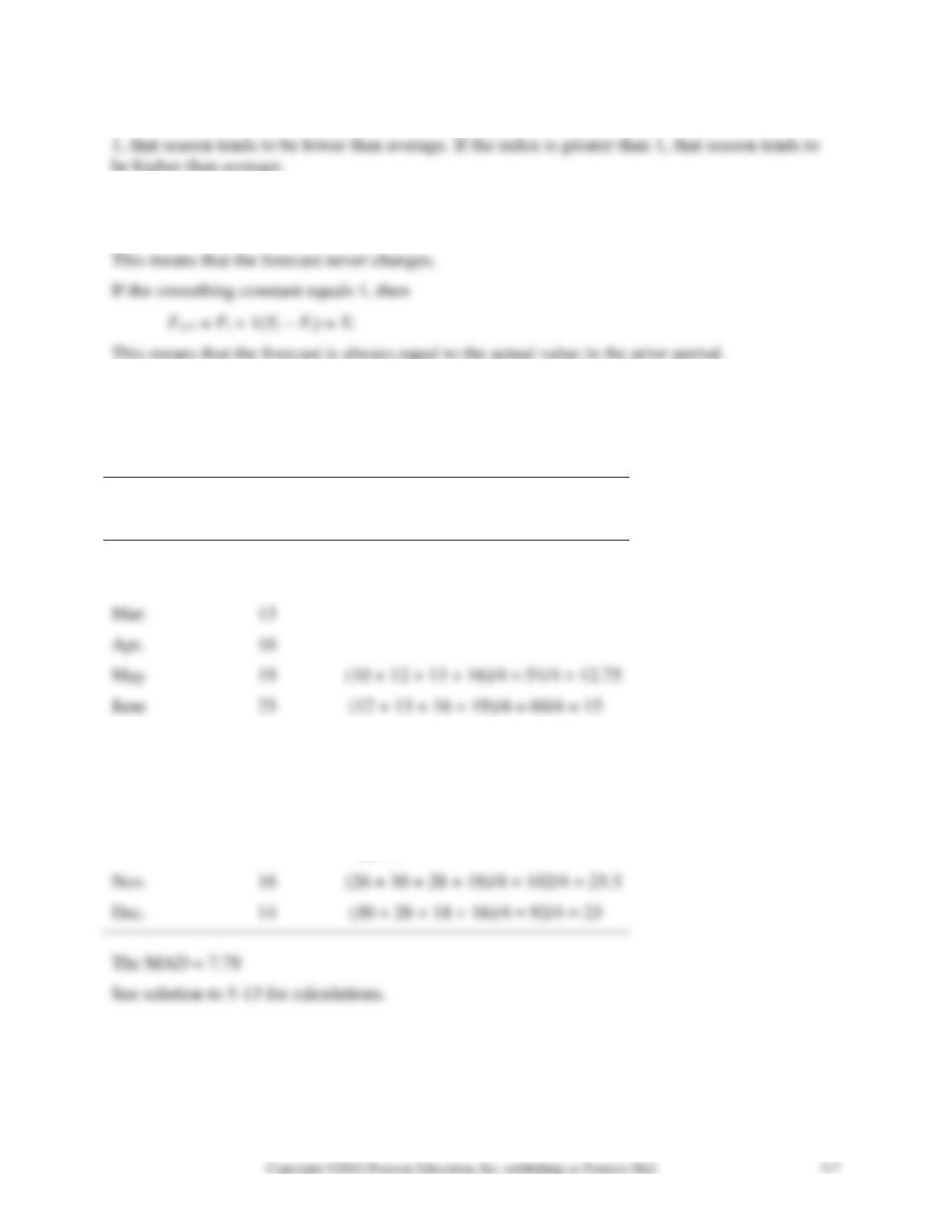
5-10. If a seasonal index equals 1, that season is just an average season. If the index is less than
5-11. If the smoothing constant equals 0, then
Ft+1 = Ft + 0(Yt − Ft) = Ft
5-12. A centered moving average (CMA) should be used if trend is present in data. If an overall
average is used rather than a CMA, variations due to trend will be interpreted as variations due to
seasonal factors. Thus, the seasonal indices will not be accurate.
5-13.
Actual
Month
Shed Sales
Four-Month Moving Average
Jan.
10
Feb.
12
Mar.
13
May
19
(10 + 12 + 13 + 16)/4 = 51/4 = 12.75
June
23
(12 + 13 + 16 + 19)/4 = 60/4 = 15
July
26
(13 + 16 + 19 + 23)/4 = 70/4 = 17.75
Aug.
30
(16 + 19 + 23 + 26)/4 = 84/4 = 21
Sept.
28
(19 + 23 + 26 + 30)/4 = 98/4 = 24.5
Oct.
18
(23 + 26 + 30 + 28)/4 = 107/4 =
26.75
Nov.
16
(26 + 30 + 28 + 18)/4 = 102/4 = 25.5
Dec.
14
(30 + 28 + 18 + 16)/4 = 92/4 = 23
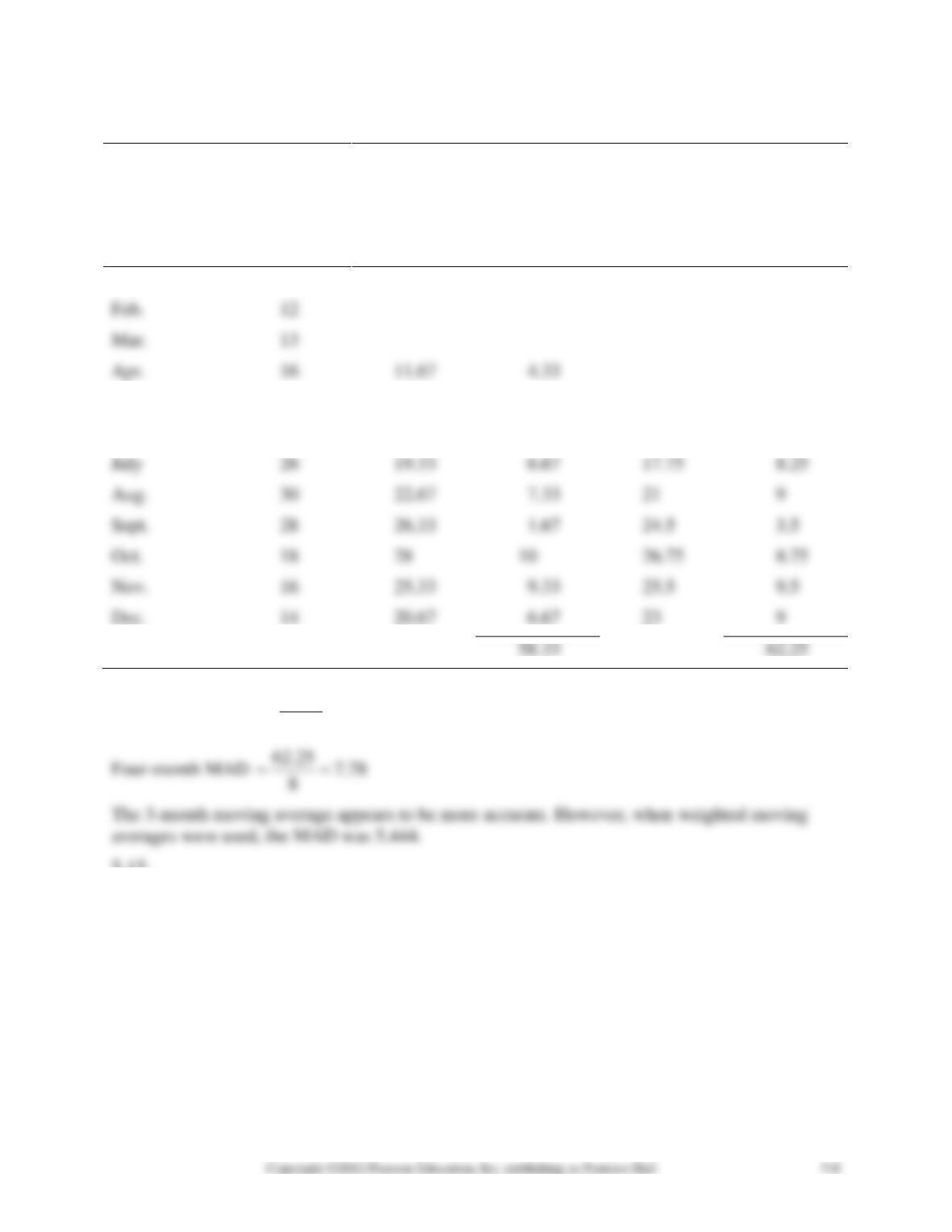
5-14.
Three-
Four-
Three-
Month
Four-
Month
Actual
Month
Absolute
Month
Absolute
Month
Shed Sales
Forecast
Deviation
Forecast
Deviation
Jan.
10
Feb.
12
Mar.
13
May
19
13.67
5.33
12.75
6.25
June
23
16
7
15
8
July
26
19.33
6.67
17.75
8.25
Aug.
30
22.67
7.33
21
9
Sept.
28
26.33
1.67
24.5
3.5
Oct.
18
28
10
26.75
8.75
Nov.
16
25.33
9.33
25.5
9.5
Dec.
14
20.67
6.67
23
9
58.33
62.25
Three-month MAD
58.33 6.48
9
==
5-15.
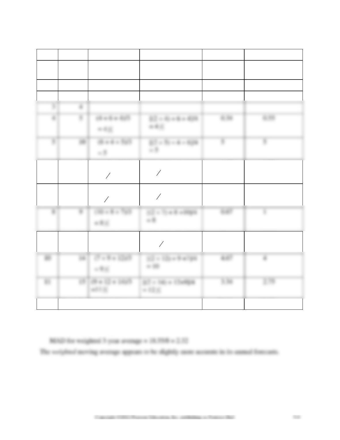
Year
Demand
3-Year Moving
Ave.
3-Year Wt. Moving
Ave.
3-Year Abs.
Deviation
3-Year Wt. Abs.
Deviation
1
4
2
6
3
4
4
5
0.34
0.55
5
10
[(2 5) + 4 + 6]/4
= 5
5
5
6
8
(4 + 5 + 10)/3
= 6
13
[(2 10) + 5 +4]/4
= 7
14
1.67
0.75
7
7
(5 + 10 + 8)/3
= 7
23
[(2 8) + 10 +5]/4
= 7
34
0.67
0.75
8
9
(10 + 8 + 7)/3
= 8
[(2 7) + 8 +10]/4
0.67
1
9
12
(8 + 7 + 9)/3
= 8
[(2 9) + 7 + 8]/4
= 8
14
4
3.75
(7 + 9 + 12)/3
= 9
13
[(2 12) + 9 +7]/4
= 10
4.67
4
14
Total absolute deviations:
20.36
18.55
MAD for 3-year average = 20.36/8 = 2.55
5-16. Using Excel or QM for Windows, the trend line is
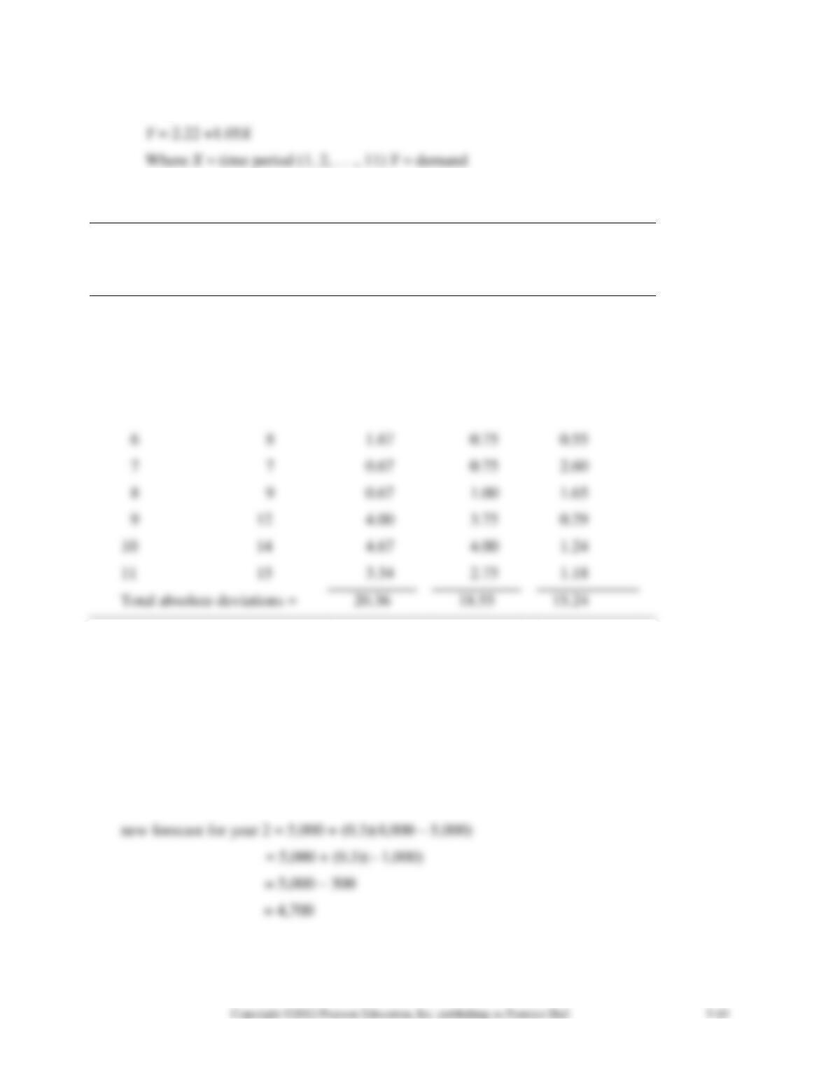
5-17. Using the forecasts in the previous problem we obtain the absolute deviations given in the
table below.
3-Yr MA
3-Yr Wt.
MA
Trend line
Year
Demand
|deviation|
|deviation|
|deviation|
1
4
—
—
0.73
2
6
—
—
1.67
3
4
—
—
1.38
4
5
0.34
0.55
1.44
5
10
5.00
5.00
2.51
6
8
1.67
0.75
0.55
7
7
0.67
0.75
2.60
8
9
0.67
1.00
1.65
9
12
4.00
3.75
0.29
10
14
4.67
4.00
1.24
11
15
3.34
2.75
1.18
Total absolute deviations =
MAD (3-year moving average) = 2.55
MAD (3-year weighted moving average) = 2.32
MAD (trend line) = 1.39
The trend line is best because the MAD for that method is lowest.
5-18. = 0.3. New forecast for year 2 is last period’s forecast + (last period’s actual demand −
last period’s forecast):
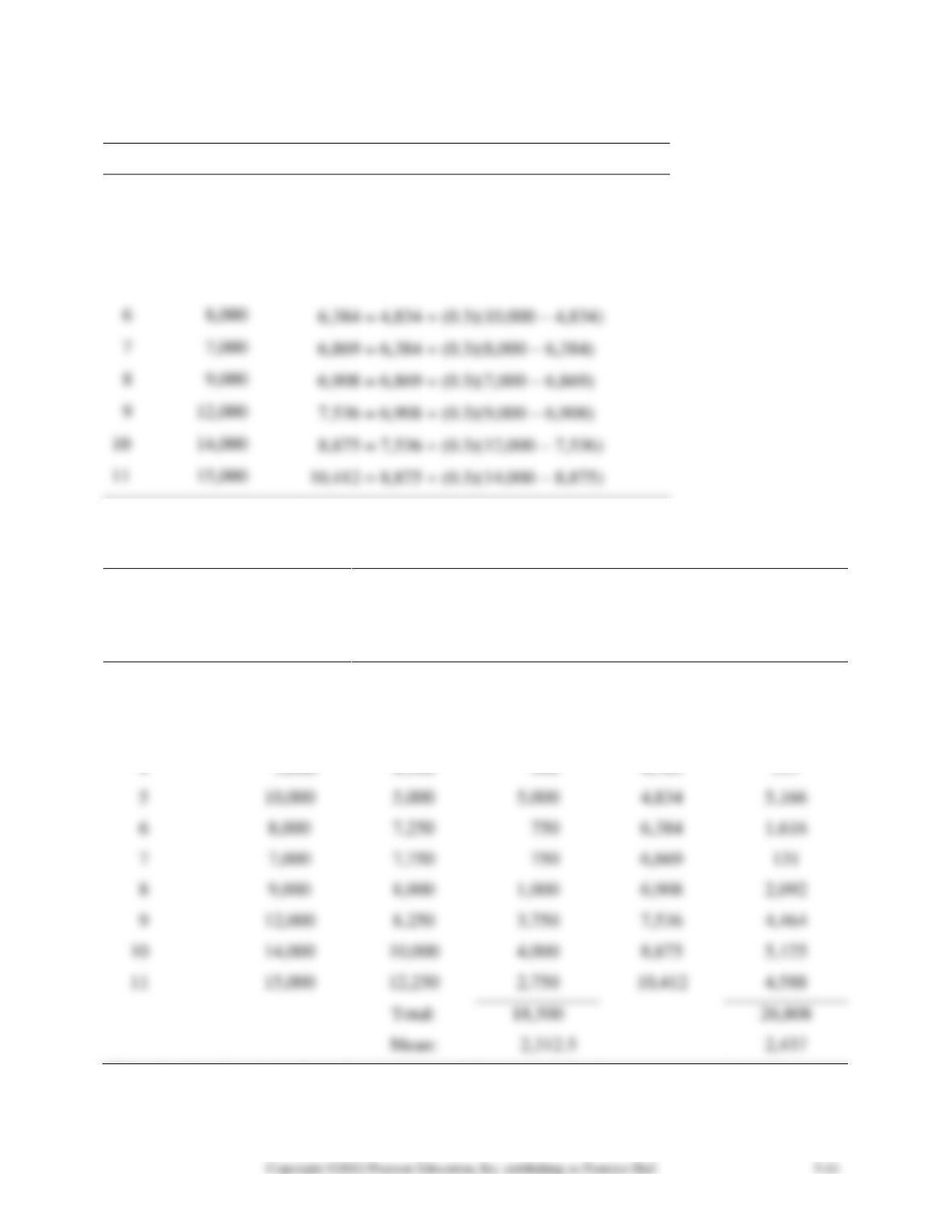
The calculations are:
Year
Demand
New Forecast
2
6,000
4,700 = 5,000 + (0.3)(4,000 − 5,000)
3
4,000
5,090 = 4,700 + (0.3)(6,000 − 4,700)
4
5,000
4,763 = 5,090 + (0.3)(4,000 − 5,090)
5
10,000
4,834 = 4,763 + (0.3)(5,000 − 4,763)
6
8,000
6,384 = 4,834 + (0.3)(10,000 − 4,834)
7
7,000
6,869 = 6,384 + (0.3)(8,000 − 6,384)
9
12,000
7,536 = 6,908 + (0.3)(9,000 − 6,908)
8,875 = 7,536 + (0.3)(12,000 − 7,536)
11
15,000
The mean absolute deviation (MAD) can be used to determine which forecasting method is more
accurate.
Weighted
Moving
Absolute
Absolute
Year
Demand
Average
Deviation
Exp. Sm.
Deviation
1
4,000
5,000
1,000
2
6,000
4,700
1,300
3
4,000
5,090
1,090
4
5,000
4,500
4,763
237
5
10,000
5,000
5,000
4,834
5,166
6
8,000
7,250
6,384
1,616
7
7,000
7,750
6,869
131
8
9,000
8,000
1,000
6,908
2,092
9
12,000
8,250
3,750
7,536
4,464
14,000
10,000
4,000
8,875
5,125
15,000
12,250
2,750
10,412
4,588
18,500
26,808
2,437
Thus, the 3-year weighted moving average model appears to be more accurate.
5-19. = 0.30
Year
1
2
3
4
5
6
Forecast
410.0
422.0
443.9
466.1
495.2
521.8
5-20.
Year
Sales
Forecast Using
= 0.6
Forecast Using
= 0.9
1
450
410
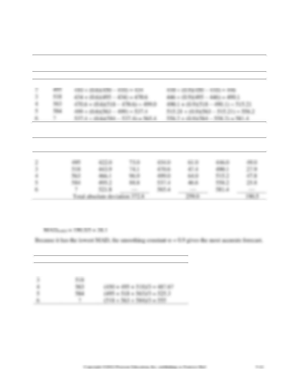
5-21.
Actual
= 0.3
Absolute
= 0.6
Absolute
= 0.9
Absolute
Year
Sales
Forecast
Deviation
Forecast
Deviation
Forecast
Deviation
1
450
410.0
40.0
410.0
40.0
410.0
40.0
2
495
422.0
73.0
434.0
61.0
446.0
49.0
3
518
443.9
74.1
470.6
47.4
490.1
27.9
4
563
466.1
96.9
499.0
64.0
515.2
47.8
5
584
495.2
88.8
537.4
46.6
558.2
25.8
6
521.8
565.4
581.4
Total absolute deviation 372.8
MAD=0.3 = 372.8/5 = 74.56
MAD=0.6 = 259/5 = 51.8
5-22.
Year
Sales
Three-Year Moving Average
1
450
2
495
3
518
4
563
5
584
6
5-23.
Time
Period
Sales
Year
X
Y
X2
XY
1
1
450
1
450
2
2
495
4
990
3
3
518
9
4
4
563
5
5
584
b1 = 33.6
b0 = 421.2
Y = 421.2 + 33.6X
5-24.
Three-Year Mov-
ing
Time-Series
Year
Actual
Sales
Average Forecast
Absolute De-
viation
Forecast
Absolute
Deviation
1
450
—
—
454.8
4.8
2
495
—
—
488.4
6.6
3
518
—
—
522.0
4.0
4
563
555.6
7.4
5
584
589.2
5.2
6
?
—
622.8
28.0
MAD=0.3 = 74.56 (see Problem 5-21)
MADmoving average = 134/2 = 67