5-16 CHAPTER 5: LINEAR EQUATIONS AND GRAPHS
Copyright © 2019 Pearson Education, Inc.
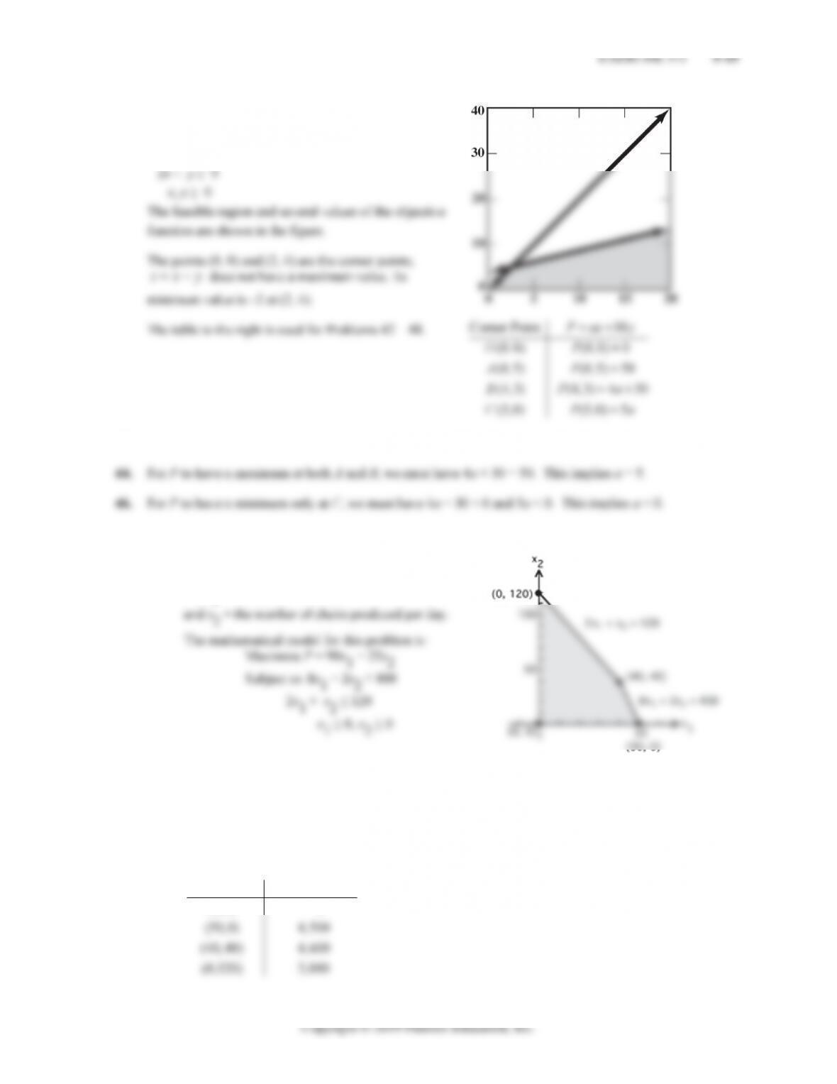
The maximum occurs at (40, 40) and the maximum value of P
is $4,600.
(B) The mathematical model for this problem is:
Maximize P = 90x1 + 25x2
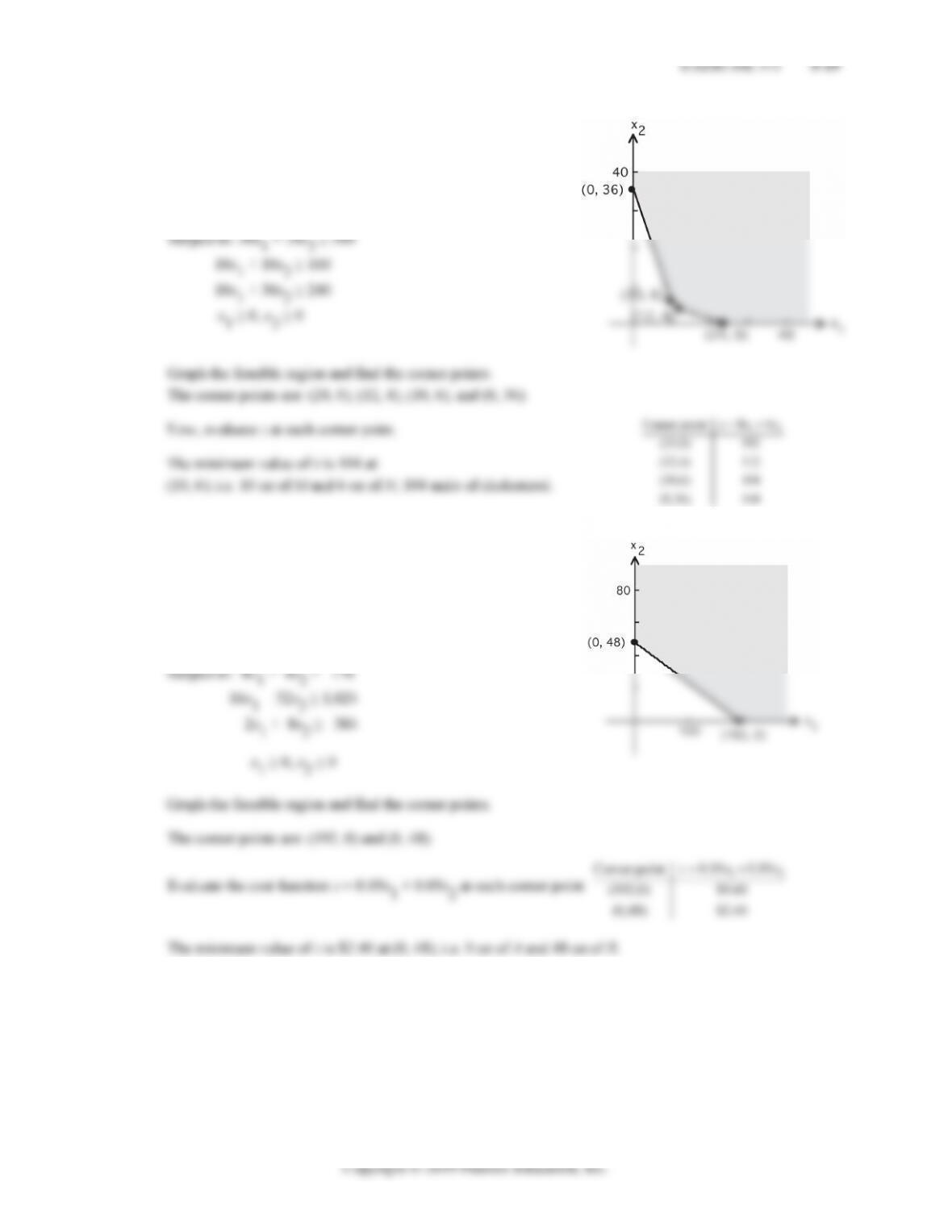
Subject to: 8x1 + 2x2 ≤ 400
The corner points are (0, 0), (20, 80), and (0, 120).
Evaluate the objective function at each corner point.
12
Corner Point 90 25
(0,0) 0
Px x
52. Summarize relevant material in table form.
(A) Standard
compute
r
Portable
compute
r
Capital expenditure $400 $250
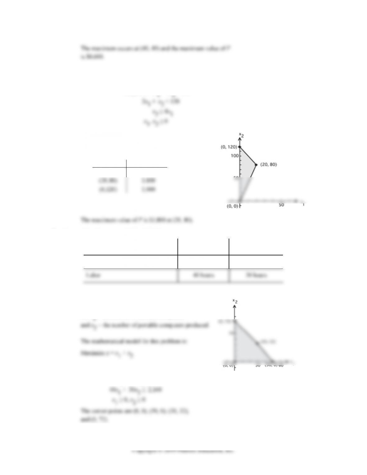
Form a mathematical model for the problem.
Let x1 = the number of standard computers
Subject to: 400x1 + 250x2 ≤ 20,000
EXERCISE 5-3 5-17
Evaluate the objective function at each corner point.
12
Corner Point
(0,0) 0
zx x
(B) Let P be the profit function. Then P = 320x1 + 220x2.
Profit on 72 portable computers
is $15,840. The maximum value of
12
Corner Point 320 220
(0,0) 0
Px x
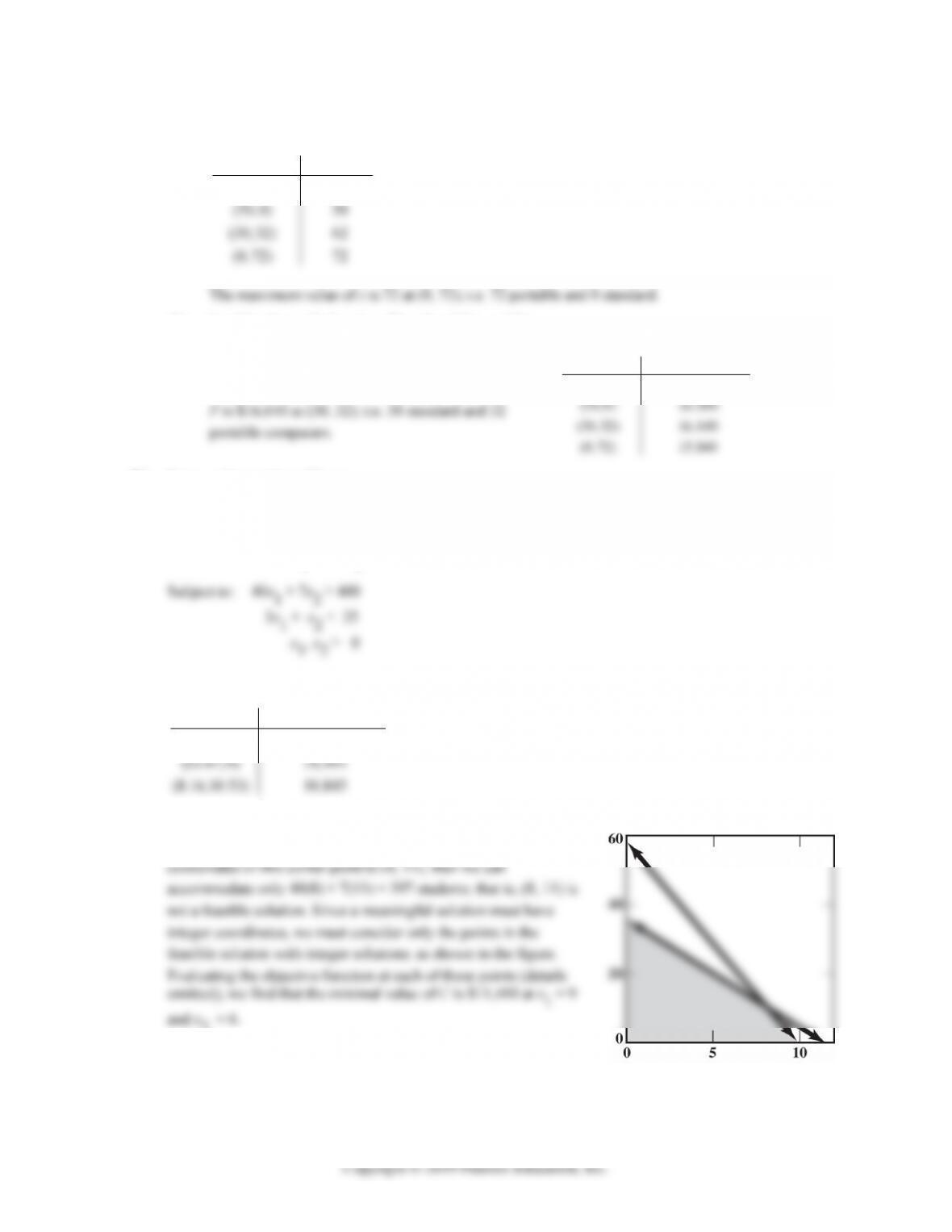
54. Let x1 = the number of buses
and x2 = the number of vans.
The changes in the data for Problem 43 change the model to:
Minimize C = 1200x1 + 100x2
Values of the objective function are shown in the table.
12
Corner Point 1200 100
(10,0) 12,000
Cxx
The minimum value of C is 10,845 at (8.16, 10.53). But decimal
solutions do not make sense in this problem. If we round the
5-18 CHAPTER 5: LINEAR EQUATIONS AND GRAPHS
56. Let x1 = amount invested in bonds of AAA quality
and x2 = amount invested in bonds of B quality.
The mathematical model for this problem is
Maximize P = 0.06x1 + 0.10x2
58. Let x1 = the number of drive-through restaurants
and x2 = the number of full-service restaurants.
The mathematical model for this problem is:
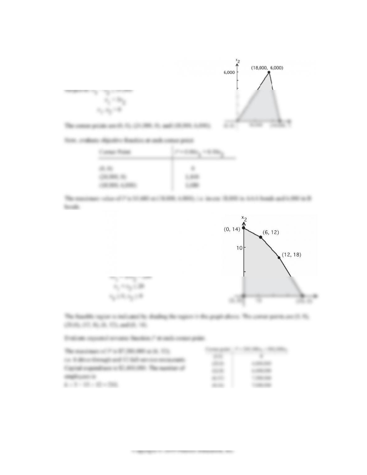
Maximize P = 200,000x1 + 500,000x2
Subject to: 100,000x1 + 150,000x2 ≤ 2,400,000
Capital expenditure is $2,400,000. The number of
employees is
6 × 5 + 15 × 12 = 210.
(12,8) 6,400,000
(6,12) 7,200,000
(0,14) 7,000,000
5-20 CHAPTER 5: LINEAR EQUATIONS AND GRAPHS
64. Let x1 = the number of Sociologists
and x2 = the number of Research assistants.
The mathematical model for this problem is:
CHAPTER 5 REVIEW
1. x > 2y – 3 or x – 2y > –3
Graph the line x – 2y = –3 as a dashed line. Substituting x = 0,
2. 3y – 5x ≤ 30
Graph the line 3y – 5x = 30 as a solid line. Substituting x = 0,
CHAPTER 5 REVIEW 5-21
3. 5x + 9y ≤ 90, x ≥ 0, y ≥ 0
The graph of 5x + 9y ≤ 90 is the half-plane below the line
4. 15x + 16y ≥ 1,200, x ≥ 0, y ≥ 0
The graph of 15x + 16y ≥ 1200 is the half-plane above the line
(5-2)
5. 2x + y ≤ 8
(5-2)
6. 3x + y ≥ 9
(5-2)
7. The boundary line passes through (6, 0) and (0, –4).
5-22 CHAPTER 5: LINEAR EQUATIONS AND GRAPHS
Copyright © 2019 Pearson Education, Inc.
Boundary line equation: y = 2
3x – 4
3y = 2x – 12
2x – 3y = 12
Since (0, 0) is in the shaded region and the boundary line is solid, the graph is the graph of 2x – 3y ≤ 12.
(5-1)
8. The boundary line passes through (2, 0) and (0, 8).
slope: m = 08
20
= –4
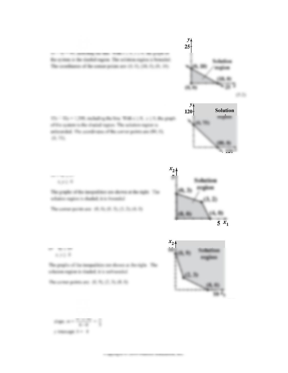
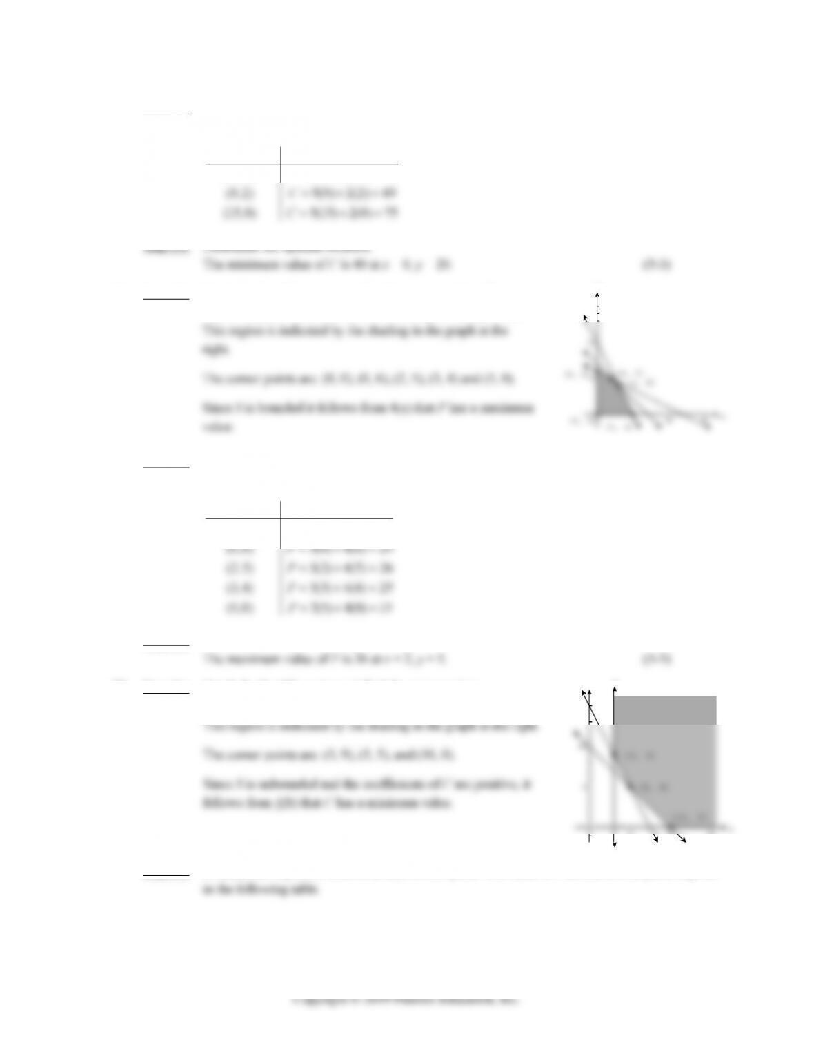
9. Step (1): Graph the feasible region and find the corner points. The
feasible region S is the solution set of the given inequalities.
This region is indicated by the shading in the graph at the right.
(4, 2), and (5, 0).
10
y
(0, 4)
Step (2): Evaluate the objective function at each corner point. The value of P at each corner point is given
in the following table.
Corner Point 2 6
Pxy
Step (3): Determine the optimal solution.
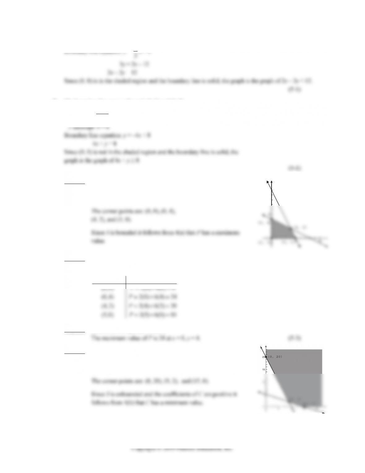
10. Step (1): Graph the feasible region and find the corner points.
The feasible region S is the solution set of the given inequalities.
This region is indicated by the shading in the graph at the right.
CHAPTER 5 REVIEW 5-23
Step (2): Evaluate the objective function at each corner point. The value of C at each corner point is given
in the following table.
Corner Point 5 2
(0,20) 5(0) 2(20) 40
Cxy
C
Step (3): Determine the optimal solution.
11. Step (1): Graph the feasible region and find the corner points. The
feasible region S is the solution set of the given inequalities.
right.
15
y
Step (2): Evaluate the objective function at each corner point. The value of P at each corner point is given
in the following table.
Corner Point 3 4
(0,0) 3(0) 4(0) 0
Pxy
P
Step (3): Determine the optimal solution.
12. Step (1): Graph the feasible region and find the corner points.
The feasible region S is the solution set of the given inequalities.
51015
15
y
(10, 0)
Step (2): Evaluate the objective function at each corner point. The value of C at each corner point is given
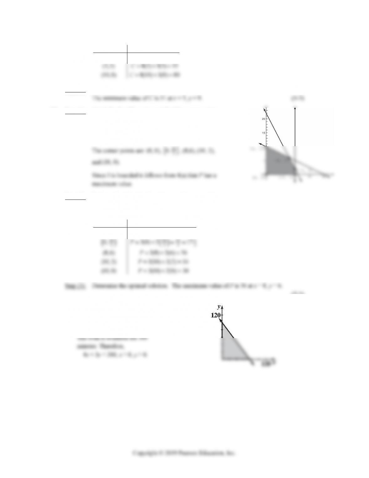
5-24 CHAPTER 5: LINEAR EQUATIONS AND GRAPHS
Corner Point 8 3
(3,9) 8(3) 3(9) 51
Cxy
C
Step (3): Determine the optimal solution.
13. Step (1): Graph the feasible region and find the corner points.
The feasible region S is the solution set of the given
inequalities. This region is indicated by the shading in the
graph at the right.
26
Step (2): Evaluate the objective function at each corner point.
The value of P at each corner point is given in the following table.
26 26 52 1
Corner Point 3 2
(0,0) 3(0) 2(0) 0
Pxy
P
(5-3)
14. Let x = number of calculator boards
y = number of toaster boards
(A) 5 hours = 5(60) = 300 minutes
CHAPTER 5 REVIEW 5-25
(B) 2 hours = 2(60) = 120 minutes
The wave machine is available for 120 minutes.
Therefore,
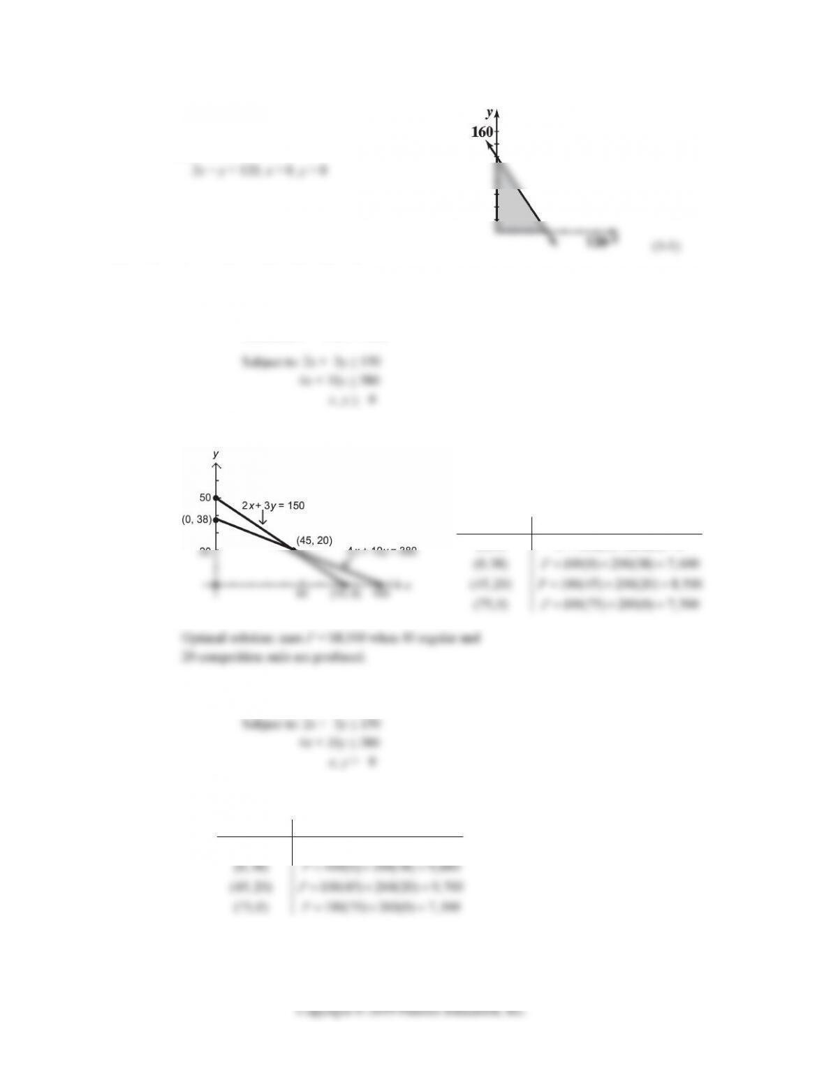
15. (A) Let x = the number of regular sails
and y = the number of competition sails.
The mathematical model for this problem is:
Maximize P = 100x + 200y
The feasible region is indicated by the shading in the graph below.
The corner points are (0, 0), (0, 38),
(45, 20), (75, 0).
The value P at each corner point is:
Corner point 100 200
(0,0) 100(0) 200(0) 0
Pxy
P
(B) The mathematical model for this problem is:
Maximize P = 100x + 260y
The feasible region and the corner points are the same as in part (A).
The value of P at each corner point is:
Corner point 100 260
(0,0) 100(0) 260(0) 0
Pxy
P
The maximum profit increases to $9,880 when 38 competition and 0 regular sails are produced.
5-26 CHAPTER 5: LINEAR EQUATIONS AND GRAPHS
(C) The mathematical model for this problem is:
Maximize P = 100x + 140y
The feasible region and the corner points are the same as in parts (A) and (B). The value of P at
each corner point is:
Corner point 100 140
(0,0) 100(0) 140(0) 0
Pxy
P
The maximum profit decreases to $7,500 when 0 competition and 75 regular sails are produced.
(5-3)
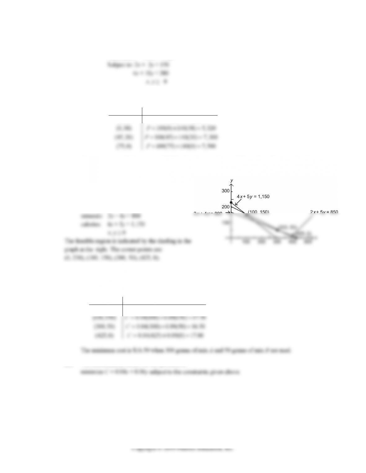
16. Let x = number of grams of mix A
y = number of grams of mix B
The constraints are:
vitamins: 2x + 5y ≥ 850
graph at the right. The corner points are:
(0, 230), (100, 150), (300, 50), (425, 0).
(A) The mathematical model for this problem is:
minimize C = 0.04x + 0.09y subject to the constraints given above.
The value of C at each corner point is:
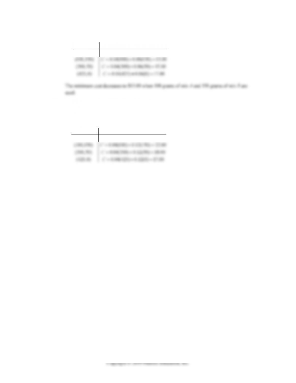
Corner point 0.04 0.09
(0, 230) 0.04(0) 0.09(230) 20.70
Cxy
C
(B) The mathematical model for this problem is:
CHAPTER 5 REVIEW 5-27
The value of C at each corner point is:
Corner point 0.04 0.06
(0, 230) 0.04(0) 0.06(230) 13.80
Cxy
C
(C) The mathematical model for this problem is:
minimize C = 0.04x + 0.12y subject to the constraints given above.
The value of C at each corner point is:
Corner point 0.04 0.12
(0, 230) 0.04(0) 0.12(230) 27.60
Cxy
C
The minimum cost increases to $17.00 when 425 grams of mix A and 0 grams of mix B are used.
(5-3)