5-25. To answer the discussion questions, two forecasting models are required: a three-period
moving average and a three-period weighted moving average. Once the actual forecasts have
been made, their accuracy can be compared using the mean absolute differences (MAD).
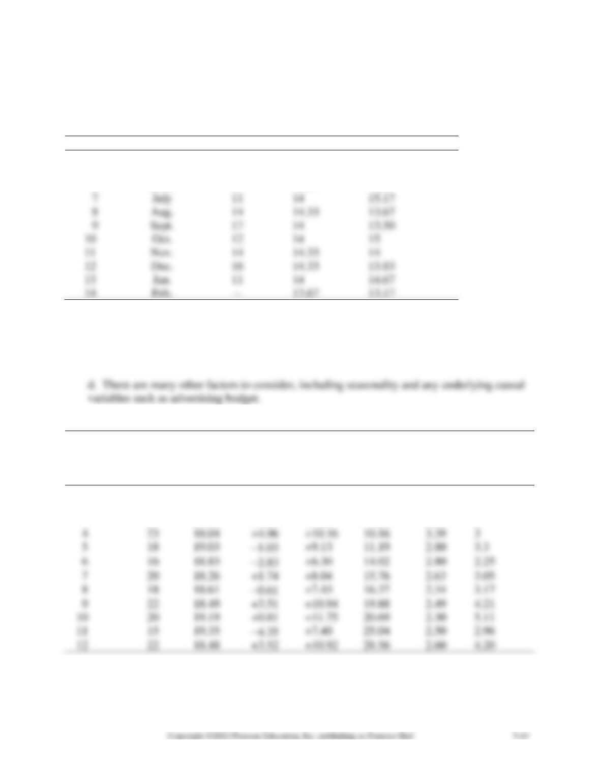
a., b. Because a three-period average forecasting method is used, forecasts start for period 4.
Period
Month
Demand
Average
Weighted Average
4
Apr.
10
13.67
14.5
5
May
15
13.33
12.67
6
June
17
13.67
13.5
7
July
11
14
15.17
8
14
14.33
13.67
9
17
14
13.50
10
Oct.
12
14
15
11
14
14.33
14
12
Dec.
16
14.33
13.83
13
11
14
14.67
14
Feb.
13.67
13.17
c. MAD for moving average is 2.2. MAD for weighted average is 2.72. Moving average
forecast for February is 13.67. Weighted moving average forecast for February is 13.17.
Thus, based on this analysis, the moving average appears to be more accurate. The forecast
for February is about 14.
5-26. a. = 0.20
Sum of
Absolute
Actual
Forecast
Forecast
Week
Miles
(Ft)
Error
RSFE
Errors
MAD
Track Signal
1
17
17.00
—
—
—
—
—
2
21
17.00
+4.00
+4.00
4.00
4.00
1
3
19
17.80
+1.20
+5.20
5.20
2.60
2
4
23
18.04
+4.96
+10.16
10.16
3.39
3
7
20
18.26
+1.74
+8.04
15.76
2.63
3.05
9
22
18.49
+3.51
+10.94
19.88
2.49
4.21
10
20
19.19
+0.81
+11.75
20.69
2.30
5.11
12
22
18.48
+3.52
+10.92
28.56
2.60
4.20
b. The total MAD is 2.60.
c. RSFE is consistently positive. Tracking signal exceeds 2 MADs at week 10. This could
indicate a problem.
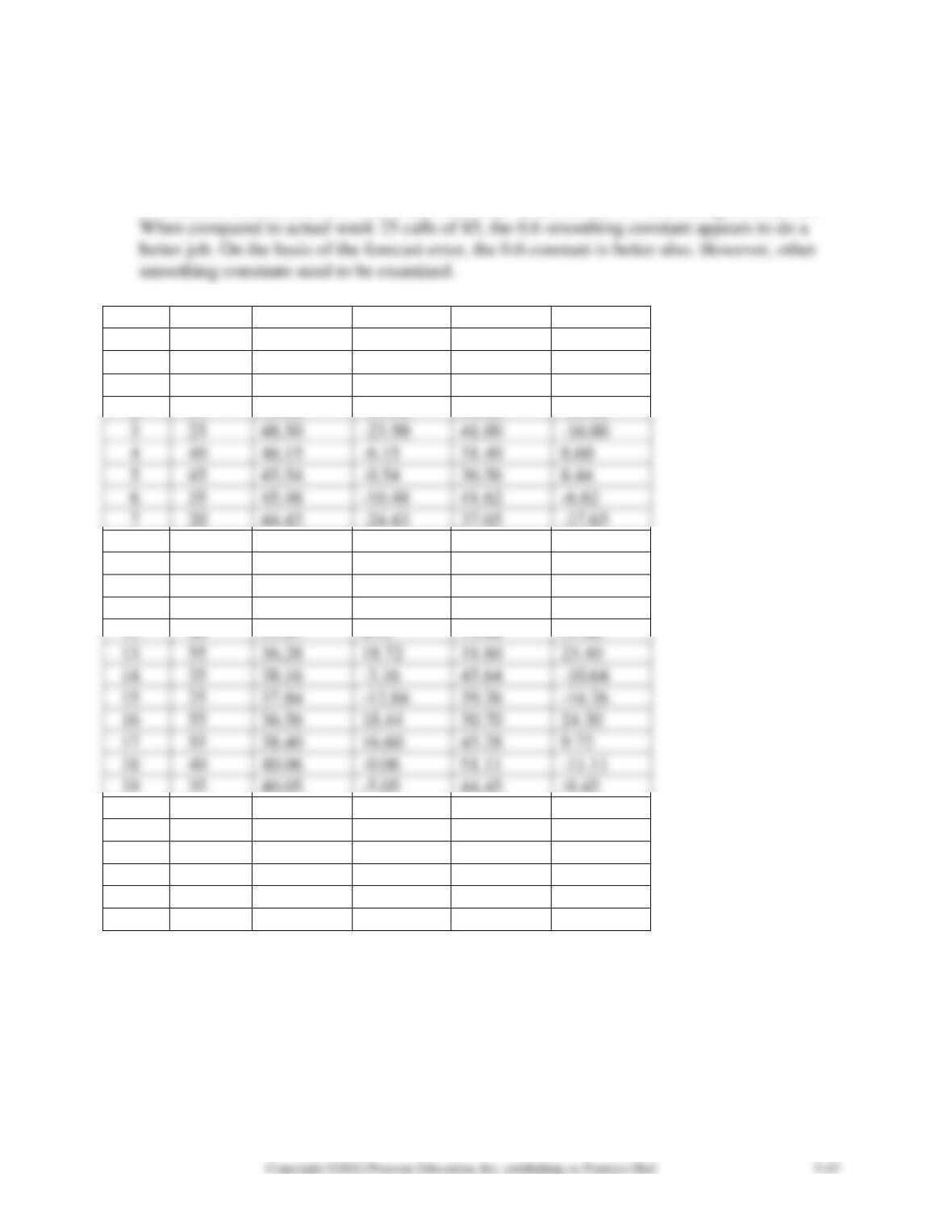
5-27. a., b. See the accompanying table for a comparison of the calculations for the exponential-
ly smoothed forecasts using constants of 0.1 and 0.6.
c. Students should note how stable the smoothed values for the 0.1 smoothing constant are.
Actual
Smoothed
Smoothed
Week,
Value,
Value,
Forecast
Value,
Forecast
t
Yt
Ft(
= 0.1)
Error
Ft(
= 0.6)
Error
1
50
50
—
—
2
35
50.00
-15.00
50.00
-15.00
3
25
48.50
-23.50
41.00
-16.00
4
40
46.15
-6.15
31.40
8.60
5
45
45.54
-0.54
36.56
8.44
6
35
45.48
-10.48
41.62
-6.62
7
20
44.43
-24.43
37.65
-17.65
8
30
41.99
-11.99
27.06
2.94
9
35
40.79
-5.79
28.82
6.18
10
20
40.21
-20.21
32.53
-12.53
11
15
38.19
-23.19
25.01
-10.01
12
40
35.87
4.13
19.00
21.00
13
55
36.28
18.72
31.60
23.40
14
35
38.16
-3.16
45.64
-10.64
15
25
37.84
-12.84
39.26
-14.26
16
55
36.56
18.44
30.70
24.30
17
55
38.40
16.60
45.28
9.72
18
40
40.06
-0.06
51.11
-11.11
19
35
40.05
-5.05
44.45
-9.45
20
60
39.55
20.45
38.78
21.22
21
75
41.59
33.41
51.51
23.49
22
50
44.93
5.07
65.60
-15.60
23
40
45.44
-5.44
56.24
-16.24
24
65
44.90
20.10
46.50
18.50
25
46.91
57.60
5-28. Using data from Problem 5-27, with = 0.9
Actual
Smoothed
Week,
Value,
Value,
Forecast
t
Yt
Ft(
= 0.9)
Error
1
50
50
—
2
35
50.00
-15.00
3
25
36.50
-11.50
4
40
26.15
13.85
5
45
38.62
6.39
6
35
44.36
-9.36
7
20
35.94
-15.94
8
30
21.59
8.41
9
35
29.16
5.84
10
20
34.42
-14.42
11
15
21.44
-6.44
12
40
15.64
24.36
13
55
37.56
17.44
14
35
53.26
-18.26
15
25
36.83
-11.83
16
55
26.18
28.82
17
55
52.12
2.88
18
40
54.71
-14.71
20
60
35.65
24.35
21
75
57.56
17.44
22
50
73.26
-23.26
23
40
52.33
-12.33
24
65
41.23
23.77
25
Note that in this problem, the initial forecast (for the first period) was not used in computing the
MAD = 14.48. Either approach is considered valid.
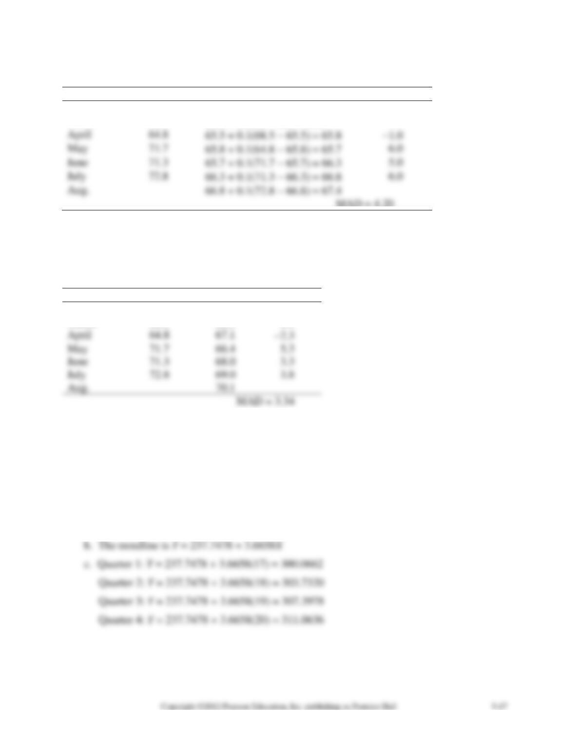
5-29. Exponential smoothing with = 0.1
Month
Income
Forecast
Error
Feb.
70.0
65.0
—
March
68.5
65.0 + 0.1(70 − 65) = 65.5
3.0
May
71.7
65.8 + 0.1(64.8 − 65.8) = 65.7
6.0
July
72.8
66.3 + 0.1(71.3 − 66.3) = 66.8
6.0
MAD = 4.20
Note that in this problem, the initial forecast (for the first period) was not used in computing the
MAD. Either approach is considered valid.
5-30. Exponential smoothing with = 0.3
Month
Income
Forecast
Error
Feb.
70.0
65.0
—
March
68.5
66.5
2.0
April
May
71.7
66.4
5.3
June
71.3
68.0
3.3
July
72.8
69.0
3.8
Based on MAD, = 0.3 produces a better forecast than = 0.1 (of Problem 5-29).
Note that in this problem, the initial forecast (for the first period) was not used in computing the
MAD. Either approach is considered valid.
5-31. Using QM for Windows, we select Forecasting – Time Series and multiplicative decompo-
sition. Then specify Centered Moving Average and we have the following results:
a. Quarter 1 index = 0.8825; Quarter 2 index = 0.9816; Quarter 3 index = 0.9712; Quarter 4
index = 1.1569
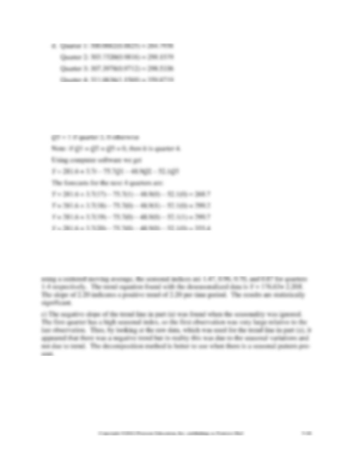
5-32. Letting
t = time period (1, 2, 3, . . . , 16)
Q1 = 1 if quarter 1, 0 otherwise
Q2 = 1 if quarter 2, 0 otherwise
5-33 a. Using computer software we get Y = 197.5 – 0.34X where X = time period.
The slope is -0.34 which indicates a small negative trend. Note that the results are not statistical-
ly significant and r2 = 0.001
b) Using QM for Windows for the multiplicative decomposition method with 4 seasons asnd
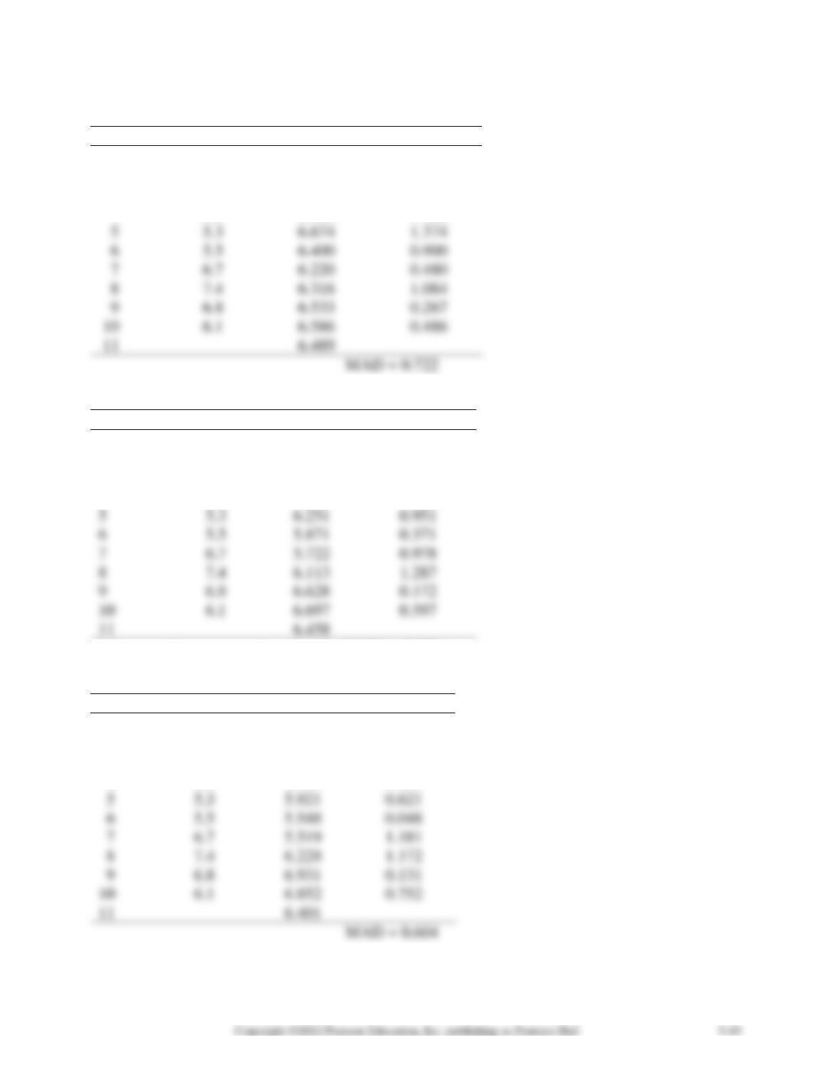
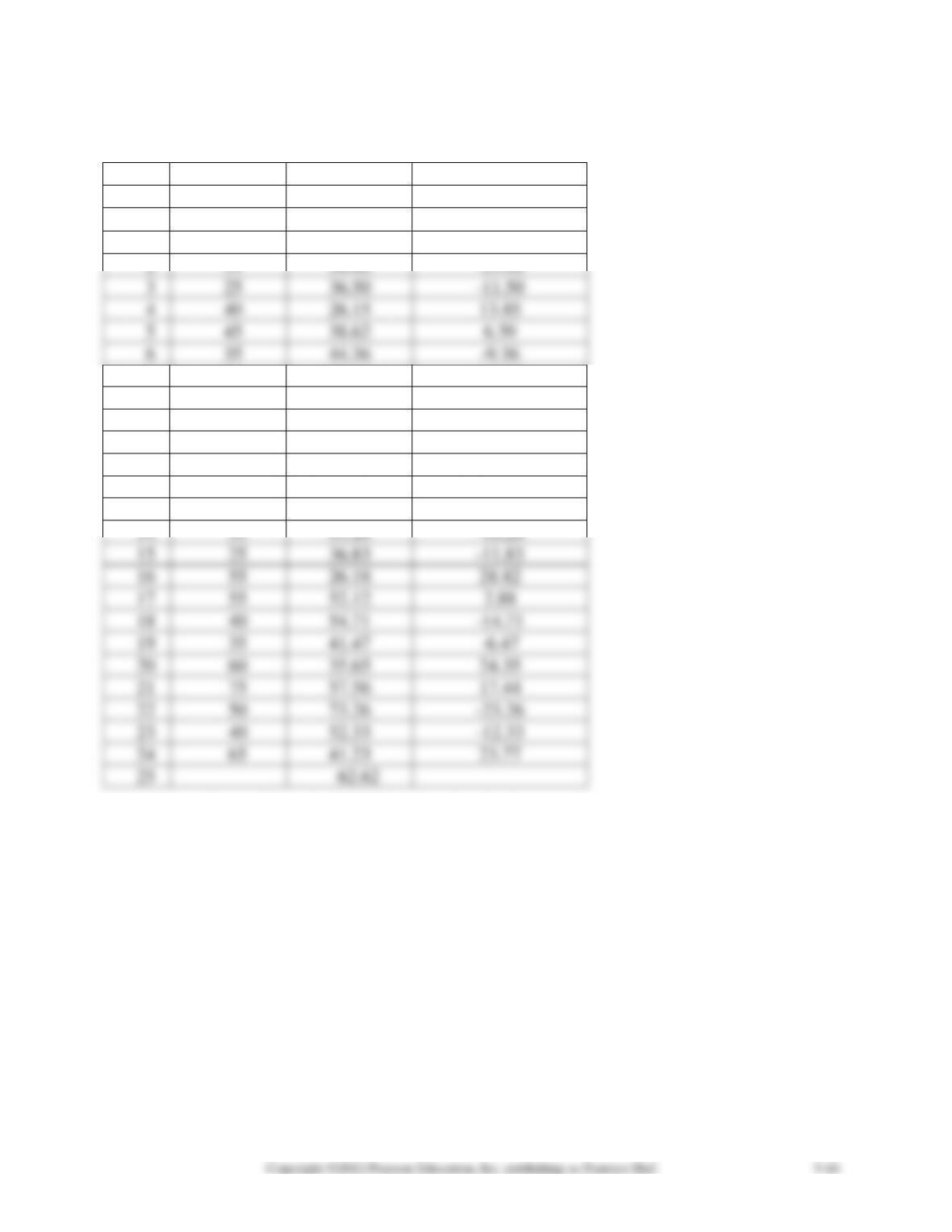
5-34. For a smoothing constant of 0.2, the forecast for year 11 is 6.489.
Year
Rate
Forecast
|Error|
1
7.2
7.2
0
2
7
7.2
0.2
3
6.2
7.16
0.96
4
5.5
6.968
1.468
5
5.3
6.674
1.374
6
5.5
6.400
0.900
7
6.7
6.220
0.480
8
7.4
6.316
1.084
9
6.8
6.533
0.267
6.1
6.586
0.486
6.489
For a smoothing constant of 0.4, the forecast for year 11 is 6.458.
Year
Rate
Forecast
|Error|
1
7.2
7.2
0
2
7
7.2
0.2
3
6.2
7.12
0.92
4
5.5
6.752
1.252
5
5.3
6.251
0.951
6
5.5
5.871
0.371
7
6.7
5.722
0.978
8
7.4
6.113
1.287
9
6.8
6.628
0.172
10
6.1
6.697
0.597
11
6.458
MAD = 0.673
For a smoothing constant of 0.6, the forecast for year 11 is 6.401.
Year
Rate
Forecast
|Error|
1
7.2
7.2
0
2
7
7.2
0.2
3
6.2
7.08
0.88
4
5.5
6.552
1.052
5
5.3
5.921
0.621
6
5.5
5.548
0.048
7
6.7
5.519
1.181
8
7.4
6.228
1.172
9
6.8
6.931
0.131
10
6.1
6.852
0.752
11
6.401
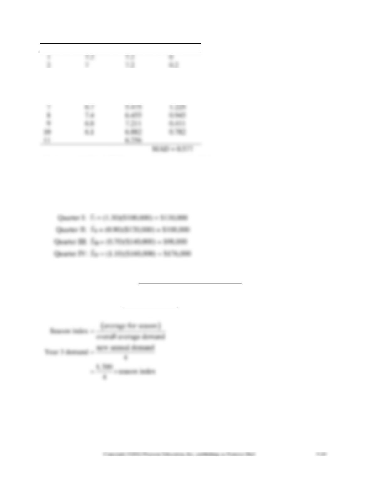
For a smoothing constant of 0.8, the forecast for year 11 is 6.256.
Year
Rate
Forecast
|Error|
1
7.2
7.2
0
2
7
7.2
0.2
3
6.2
7.04
0.84
4
5.5
6.368
0.868
5
5.3
5.674
0.374
6
5.5
5.375
0.125
7
6.7
5.475
1.225
8
7.4
6.455
0.945
9
6.8
7.211
0.411
6.1
6.882
0.782
6.256
The lowest MAD is 0.577 for a smoothing constant of 0.8.
5-35. To compute a seasonalized or adjusted sales forecast, we just multiply each seasonal index
by the appropriate trend forecast.
Ŷ = seasonal index Ŷtrend forecast
Hence for:
5-36.
(Average demand for season)
( ) ( )
year 1 demand year 2 demand
2
+
=
Overall average demand =
( )
sum of all values
8
Solution Table for Problem 5-36
Average
Year 1
Year 2
(Average Year
1-
Season
Season
Year 3
Season
Demand
Demand
Year 2 Demand)
Demand
Index
Demand
Fall
200
250
225.0
250
0.90
270
Winter
350
300
325.0
250
1.30
390
Spring
150
165
157.5
250
0.63
189
Summer
300
285
292.5
250
1.17
351
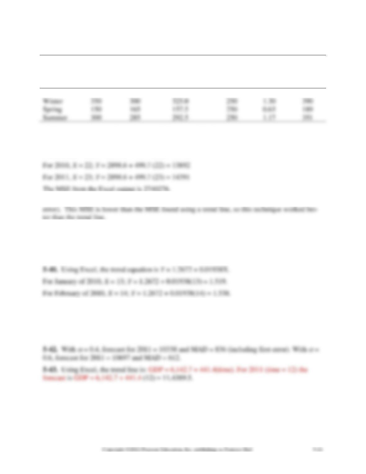
5-37. Using Excel with X = 1, 2, 3, …, 20 for years 1991-2010 respectively, the trend equation
is Y = 2898.6 + 499.7X.
For 2009, X = 21; Y = 2898.6 + 499.7 (21) = 13392
5-38. Using QM for Windows, the forecast is 10229 and the MSE = 2676625 (ignoring the first
5-39. a. With a smoothing constant of 0.4, the forecast for 2011 is 10609 with MSE =
3703109.(ignoring the first error)
b. Using QM for Windows, the best smoothing constant is 0.92. This gives the lowest MSE
of 2514990.
5-41. The forecast for January 2010 would be 1.452.
The MSE with the trend equation is 0.00049. The MSE with this exponential smoothing model is
0.00268.
SOLUTIONS TO INTERNET HOMEWORK PROBLEMS
5-44. The trend line found using Excel is: Patients = 29.73 + 3.28(time). Note these coefficients are
rounded. For the next 3 years (time = 11, 12, and 13) the forecasts for the number of patients are:
The coefficient of determination is 0.85, so the model is a fair model.
5-45. The trend line found using Excel is: Crime Rate = 51.98 + 6.09(time). Note these coeffi-
cients are rounded. For the next 3 years (time = 11, 12, and 13) the forecasts for the crime rates are:
Crime Rate = 51.98 + 6.09(11) = 118.97
Crime Rate = 51.98 + 6.09(13) = 131.15
The coefficient of determination is 0.96, so this is a very good model.
5-46. The regression equation (from Excel) is: Patients = 1.23 + 0.54(crime rate). Note these co-
efficients are rounded. If the crime rate is 131.2, the forecast number of patients is:
The coefficient of determination is 0.90, so this is a good model.
5-47. With
= 0.6, forecast for 2003 = 86.2 and MAD = 3.42. With
= 0.2, forecast for 2003 =
63.87 and MAD = 7.23. The model with
= 0.6 is better since it has a lower MAD.
Deposits = –18.968 + 1.638(45) = 54.7
Deposits = –18.968 + 1.638(46) = 56.4
Deposits = –18.968 + 1.638(47) = 58.0
The trend line (coefficients from Excel are rounded) for GSP is:
5-50. The regression equation from Excel is
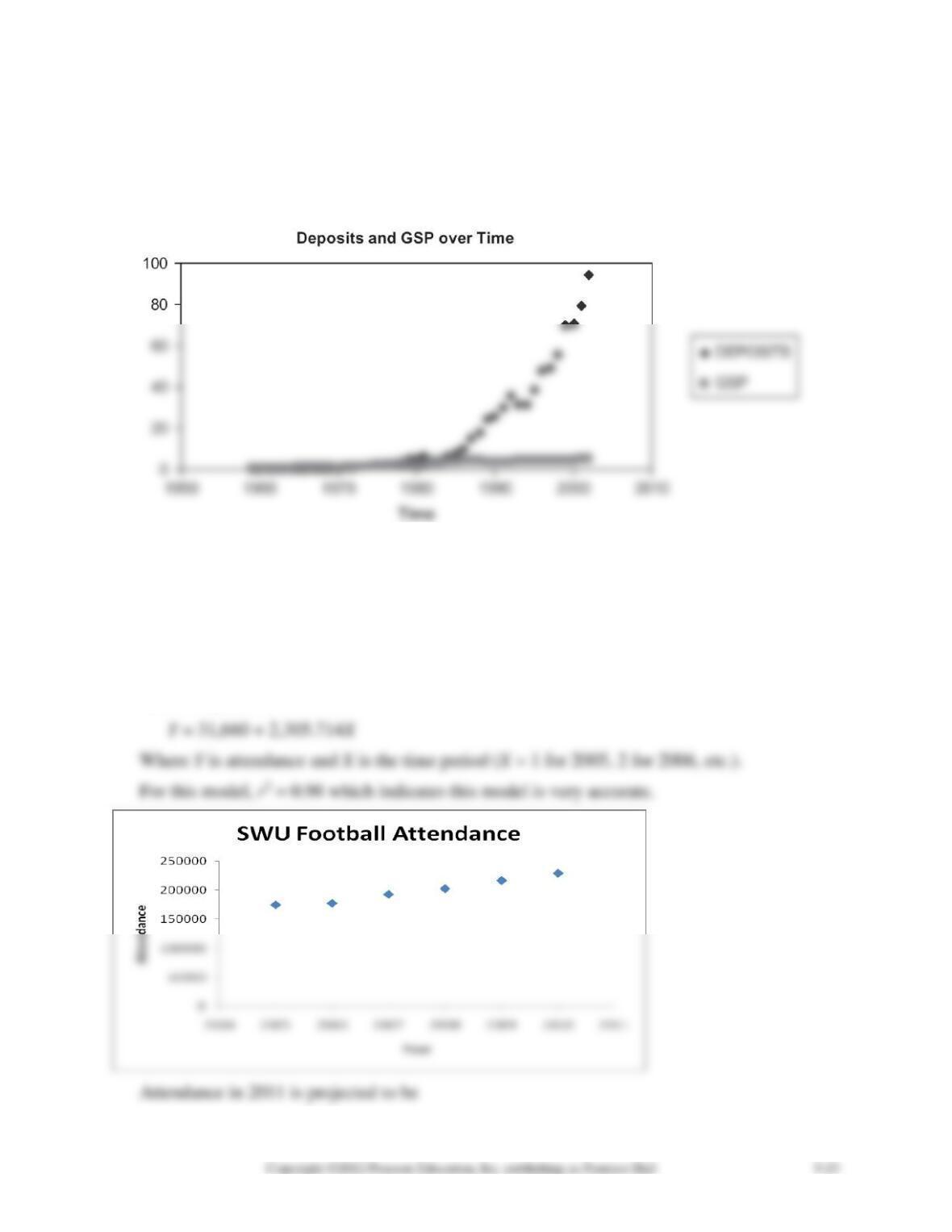
Deposits = –17.64 + 13.59(GSP)
In the scatterplot of this data that follows, the pattern appears to change around 1985. There are
definitely different relationships before 1985 and after 1985, so perhaps the model should be de-
veloped with 1985 as the first year of data.
CASE STUDIES
FORECASTING ATTENDANCE AT SWU FOOTBALL GAMES
1. Because we are interested in annual attendance and there are six years of data, we find the
average attendance in each year shown in the table below. A graph of this indicates a linear
trend in the data. Using Trend Analysis in the forecasting module of QM for Windows we
find the equation:
2014.
Year
2005
2006
2007
2008
2009
2010
Attendance
34840
35380
38520
40500
43320
45820
2. Based upon the projected attendance and tickets prices of $20 in 2011 and $21 (a 5% in-
crease) in 2012, the projected revenues are:
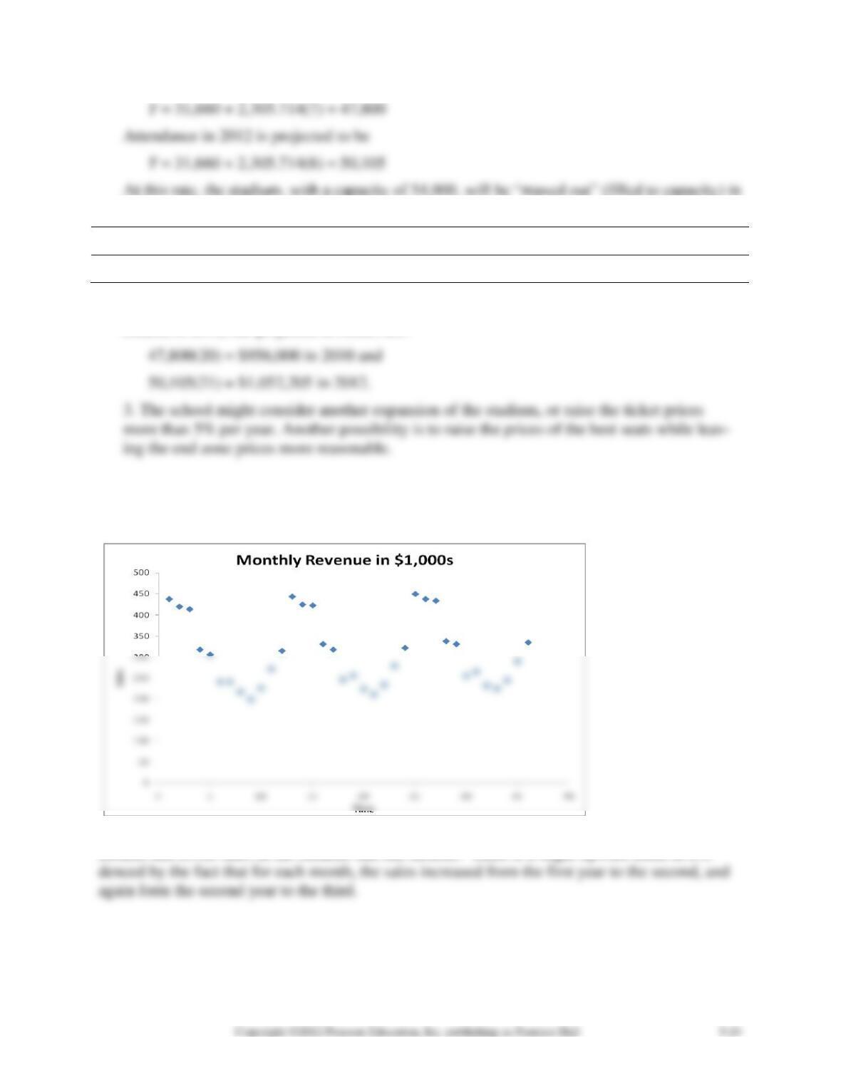
FORECASTING MONTHLY SALES
1.
The scatter plot of the data shows a definite seasonal pattern with higher sales in the winter
months and lower sales in the summer and fall months. There is a slight upward trend as evi-
2. A trend line based on the raw data is found to be:
Y = 330.889 – 1.162X
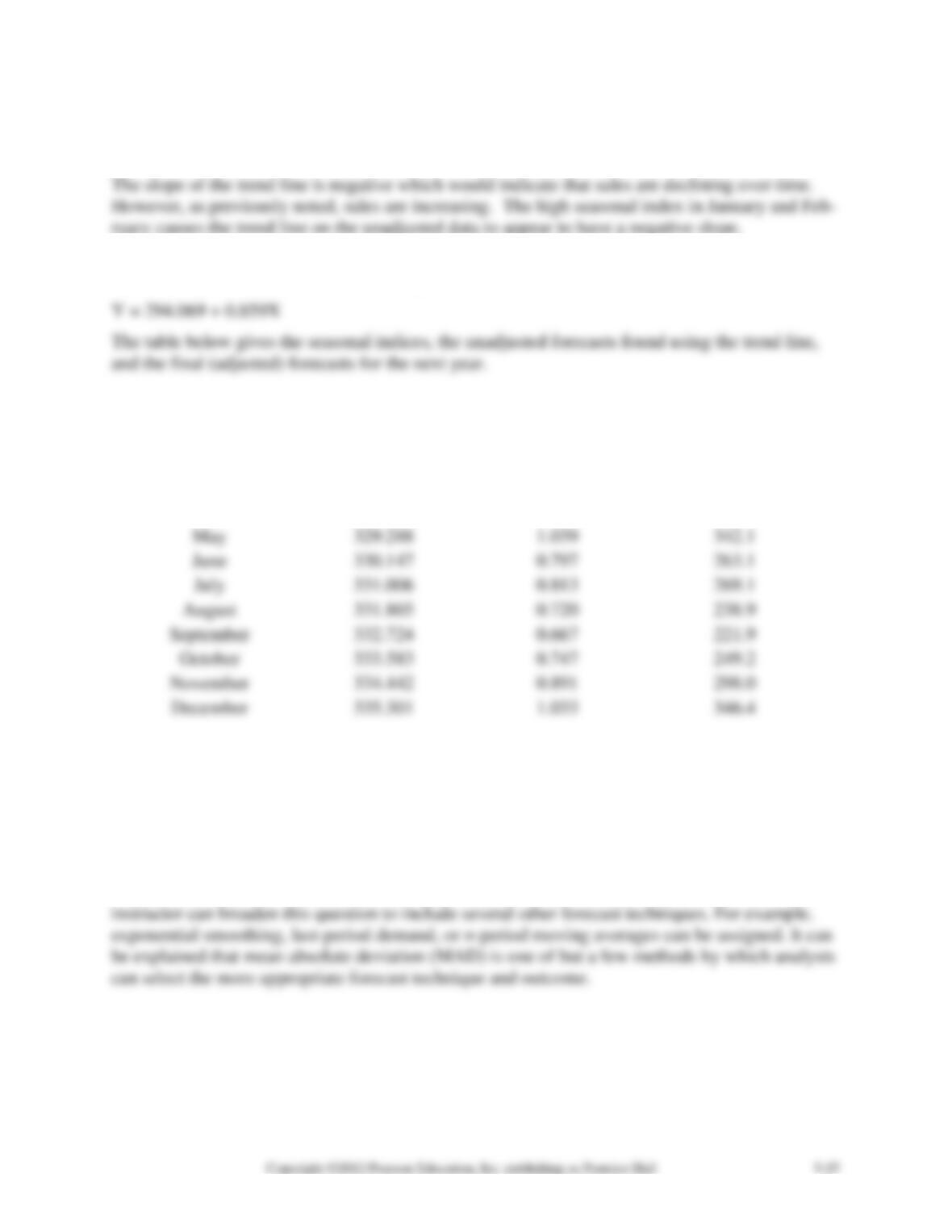
3. There is a definite seasonal pattern and a definite trend in the data. Using the decomposition
method in QM for Windows, the trend equation (based on the deseasonalized data) is
Month
Unadjusted forecast
Seasonal index
Adjusted forecast
January
325.852
1.447
471.5
February
326.711
1.393
455.1
March
327.57
1.379
451.7
April
328.429
1.074
352.7
329.288
1.039
342.1
330.147
0.797
263.1
331.006
0.813
269.1
August
331.865
0.720
238.9
332.724
0.667
221.9
October
333.583
0.747
249.2
334.442
0.891
298.0
335.301
1.033
346.4
SOLUTION TO INTERNET CASES
SOLUTION TO AKRON ZOOLOGICAL PARK CASE
1. The instructor can use this question to have the student calculate a simple linear regression,
using real-world data. The attendance would be the dependent variable and time would be the
independent variable. From the attendance, the expected revenues could be determined. Also, the
r = 0.88
MAD = 9,662
2. The student should respond that the other factors are the variability of the weather, the special
events, the competition, and the role of advertising.