4 SYSTEMS OF LINEAR EQUATIONS; MATRICES
EXERCISE 4-1
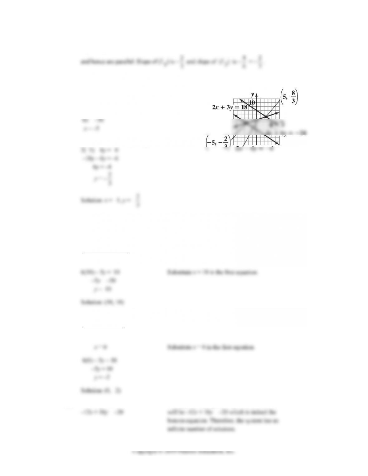
4. Set x = 0. Then y =18; (0, 18)
8. Slope = 420 16 2; 20 2( 3)
53 8 yx
14. 3x – 2y = 12
16. 3u + 5v = 15
18. y = x – 4 (1)
x + 3y = 12 (2)
By substituting y from (1) into (2), we get:
20. 3x – y = 7 (1)
2x + 3y = 1 (2)
Solve (1) for y to obtain:
22. 2x – 3y = –8 (1)
5x + 3y = 1 (2)
Add (1) and (2):
24. 2x + 3y = 1 (1)
3x – y = 7 (2)
Multiply (2) by 3 and add to (1) to obtain:
4-2 CHAPTER 4: SYSTEMS OF LINEAR EQUATIONS; MATRICES
26. 3x + 9y = 6 (1)
4x – 3y = 8 (2)
28. –5x + 15y = 10 (1)
5x – 15y = 10 (2)
30. –5x + 15y = 10 (1)
32. 5m – 7n = 9 (1)
2m – 12n = 22 (2)
34. x + y = 1 (1)
0.4x + 0.7y = 0.1 (2)
36. Here the solution is the intersection of the vertical line x = –4 and the horizontal line y = 9. These lines
38. The first equation is equivalent to 67x, so 7
6
x. The second equation is equivalent to 49y,
9
4
40. These equations give the graphs of the lines 2yxand 5yx. Those lines only intersect at (0, 0).
48.
If m = 0, then y = b. The line ynxc
intersects the horizontal line y = b exactly once, provided
50. Graphing these equations shows that they intersect at x = 1.25, y = –6.75
EXERCISE 4-1 4-3
52. y = –1.7x + 2.3
54. 3x – 7y = –20
2x + 5y = 8
y = – 2
5x + 8
5
56. First solve each equation for y:
or
x = 1.232 y = –3.347 or (1.232, –3.347).
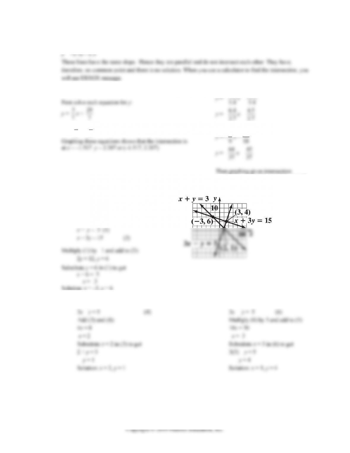
58. x + y = 3 (L1)
x + 3y = 15 (L2)
3x – y = 5 (L3)
(A) L1 and L2 intersect:
(B) L1 and L3 intersect:
x + y = 3 (3)
(C) L2 and L3 intersect:
x + 3y = 15 (5)
EXERCISE 4-1 4-5
(B) L1 and L3 do not intersect, since they have the same slope
(C) L2 and L3 intersect:
2x – 6y = –6 (3)
4x + 6y = –24 (4)
Add (3) and (4) to obtain:
Substitute x = –5 in (3) to get
64. (A) 6x – 5y = 10 Multiply the top equation by 11 and the bottom
–13x + 11y = –20 equation by 5.
66x – 55y = 110 Add the equations.
65 55 100xy
x = 10
(B) 6x – 5y = 10 Multiply the top equation by 2 and add to the
13 10 20xy
bottom equation.
–x = 0
(C) 6x – 5y = 10 Multiply the top equation by –2. The result
4-6 CHAPTER 4: SYSTEMS OF LINEAR EQUATIONS; MATRICES
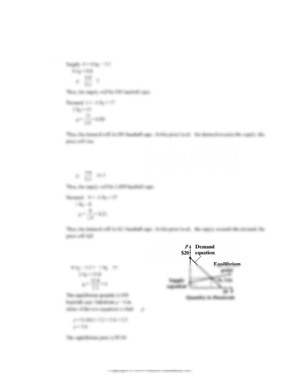
66. p = 0.4q + 3.2 Supply equation
p = –1.9q + 17 Demand equation
(A) p = $4
(B) p = $9
Supply: 9 = 0.4q + 3.2
0.4q = 5.8
(C) Solve the pair of equations to (D)
find the equilibrium price and
the equilibrium quantity.
baseball caps. Substitute q = 6 in
either of the two equations to find p.
p = 0.4(6) + 3.2 = 2.4 + 3.2
p = 5.6
The equilibrium price is $5.60.
EXERCISE 4-1 4-7
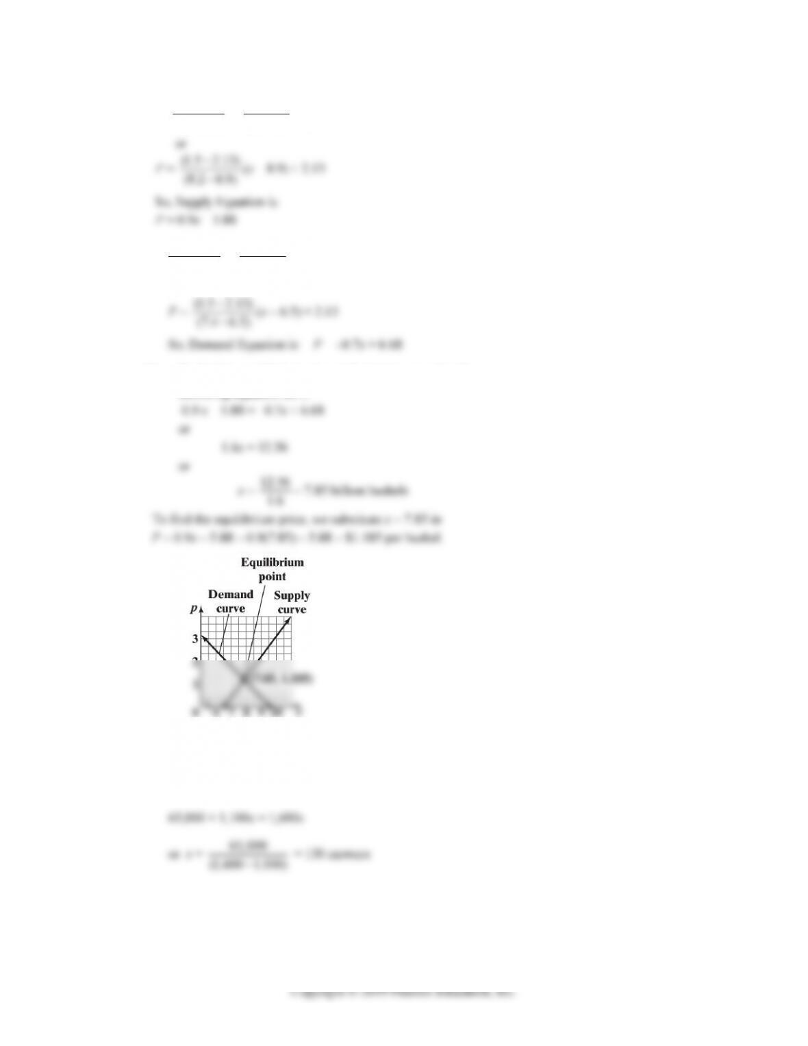
68. (A) 2.13
1.5 2.13
P
= 8.9
8.2 8.9
x
(B) 2.13
1.5 2.13
P
= 6.5
7.4 6.5
x
or
(C) To find the equilibrium price and quantity, we solve the
following equation for x:
(D)
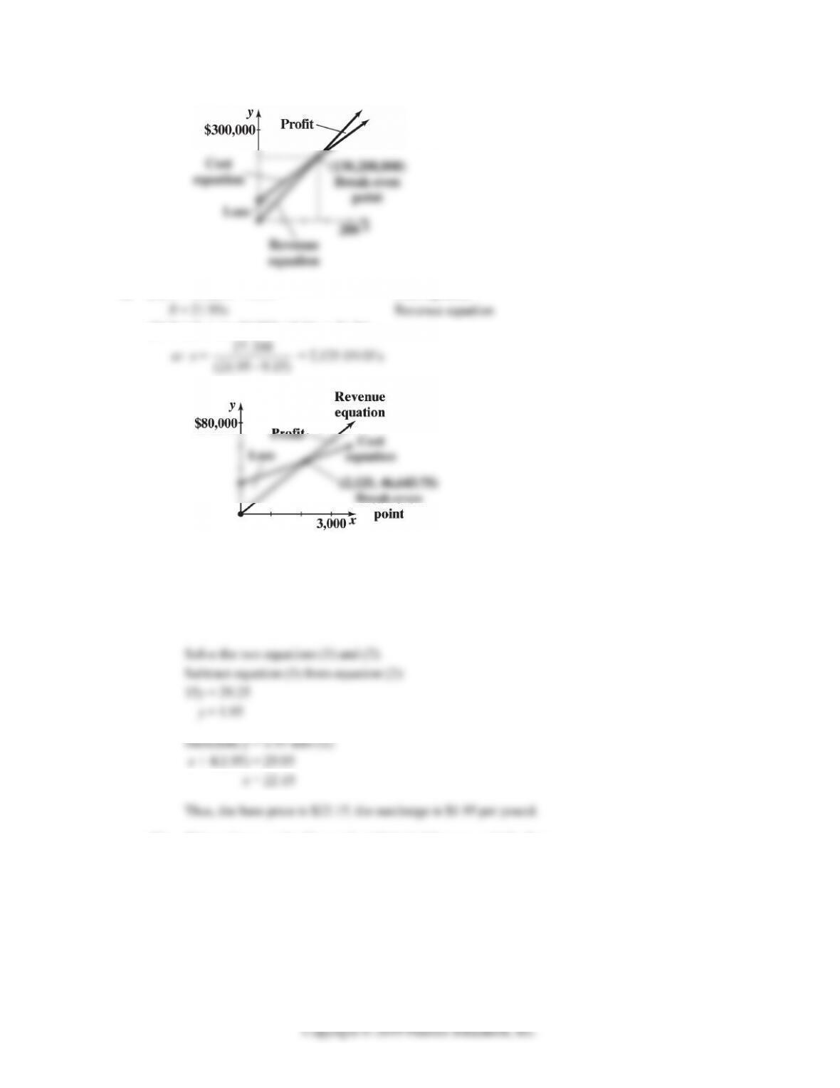
70. y = 65,000 + 1,110x Revenue equation
y = 1,600x Cost equation
(A) To break even, we need to solve the following equation:
4-8 CHAPTER 4: SYSTEMS OF LINEAR EQUATIONS; MATRICES
(B)
72. (A) C = 27,200 + 9.15x Cost equation
(B) Break even: 27,200 + 9.15x = 21.95x
(C)
74. Let x = base price
y = surcharge
(A) 5 pound package: x + 4y = 29.95 (1)
20 pound package: x + 19y = 59.20 (2)
(B) Ship packages under 10 pounds with United Express and all others
with the Federated Shipping.
EXERCISE 4-1 4-9
76. (A) Total amount of Columbian beans: 132 × 50 = 6,600 lbs.
Total amount of Brazilian beans: 132 × 40 = 5,280 lbs.
To make a pound of mild blend, we need 6
16 pound of Columbian beans
(B) To produce a pound of robust blend, we need 12
16 pound of Columbian beans and 4
16 pound of
78. Let x = number of bags of Brand A fertilizer needed, and
y = number of bags of Brand B fertilizer needed.
–5y = –280
y = 56
80. Let x and y be the number of production hours of Green Bay plant and Sheboygan plant. Then
xy
xy
4-10 CHAPTER 4: SYSTEMS OF LINEAR EQUATIONS; MATRICES
Copyright © 2019 Pearson Education, Inc.
or y = 142.5
5 = 28.5 hours
Substituting this value for y in 8x + 5y = 622.5, we obtain x:
8x + 5(28.5) = 622.5
or x = 622.5 5(28.5)
8
= 60 hours.
82. We have s = a + bt2 and for t = 1, s = 240 and for t = 2, s = 192.
(A) We note that
2
240 (1)
ab ab
b
16
84. Let t1 and t2 be the time recorded in water and air respectively. Then
21
21
6
1,100 5,000
tt
tt
or
21
21
6
50
11
tt
tt
(A) Substituting t2 from the second equation into the first equation, we obtain:
(B) 5,000 22
13
≈ 8,462 ft.
EXERCISE 4-2
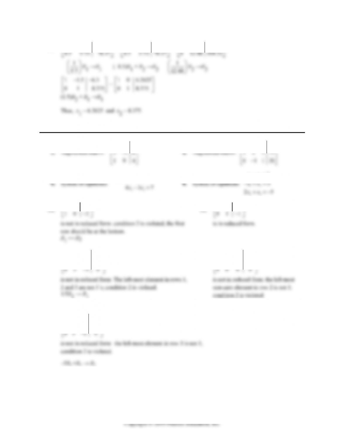
16. Coefficient matrix: 83
; augmented matrix: 8310
EXERCISE 4-2 4-11
Copyright © 2019 Pearson Education, Inc.
20. 2
315
x
212
xx
24. Interchange rows 1 and 2.
135
26. Multiply row 2 by –2.
24 6
28. Replace row 2 by the
sum of row 1 and row 2.
3711
30. Multiply row 1 by 1
2
32. Replace row 1 by the sum of row
34. Replace row 2 by the
44. 12 5
2410
2R1 + R2 → R2 125
000
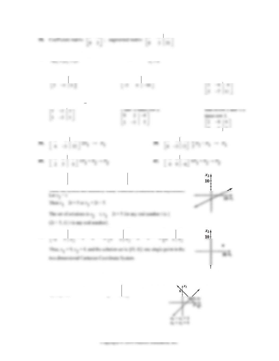
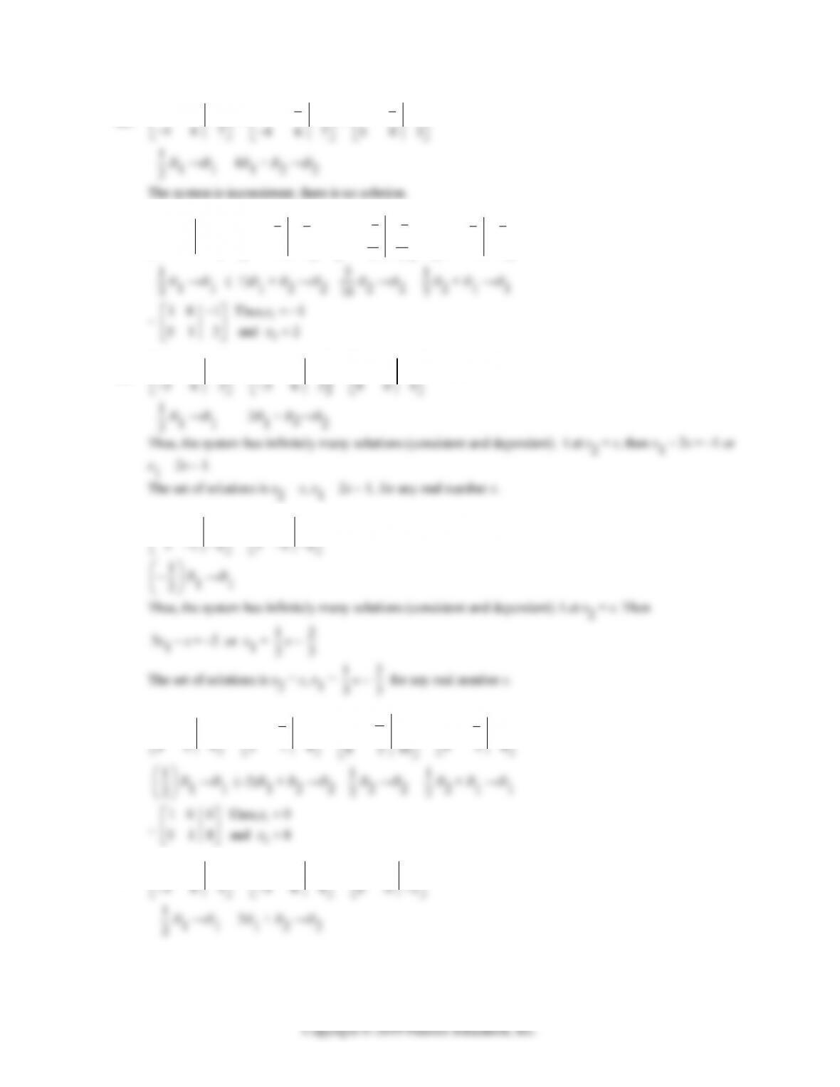
The set of solutions is x2 = t, x1 = 2t + 5 for any real number t is {
(2t + 5, t) | t is any real number}.
46. 121
2R1 + R2 → R2 121
2R2 + R1 → R1 109
48. System Augmented matrix Graphs:
12
2
6
xx
xx
112
4-12 CHAPTER 4: SYSTEMS OF LINEAR EQUATIONS; MATRICES
Copyright © 2019 Pearson Education, Inc.
112
116
(–1)R1 + R2 → R2 112
024
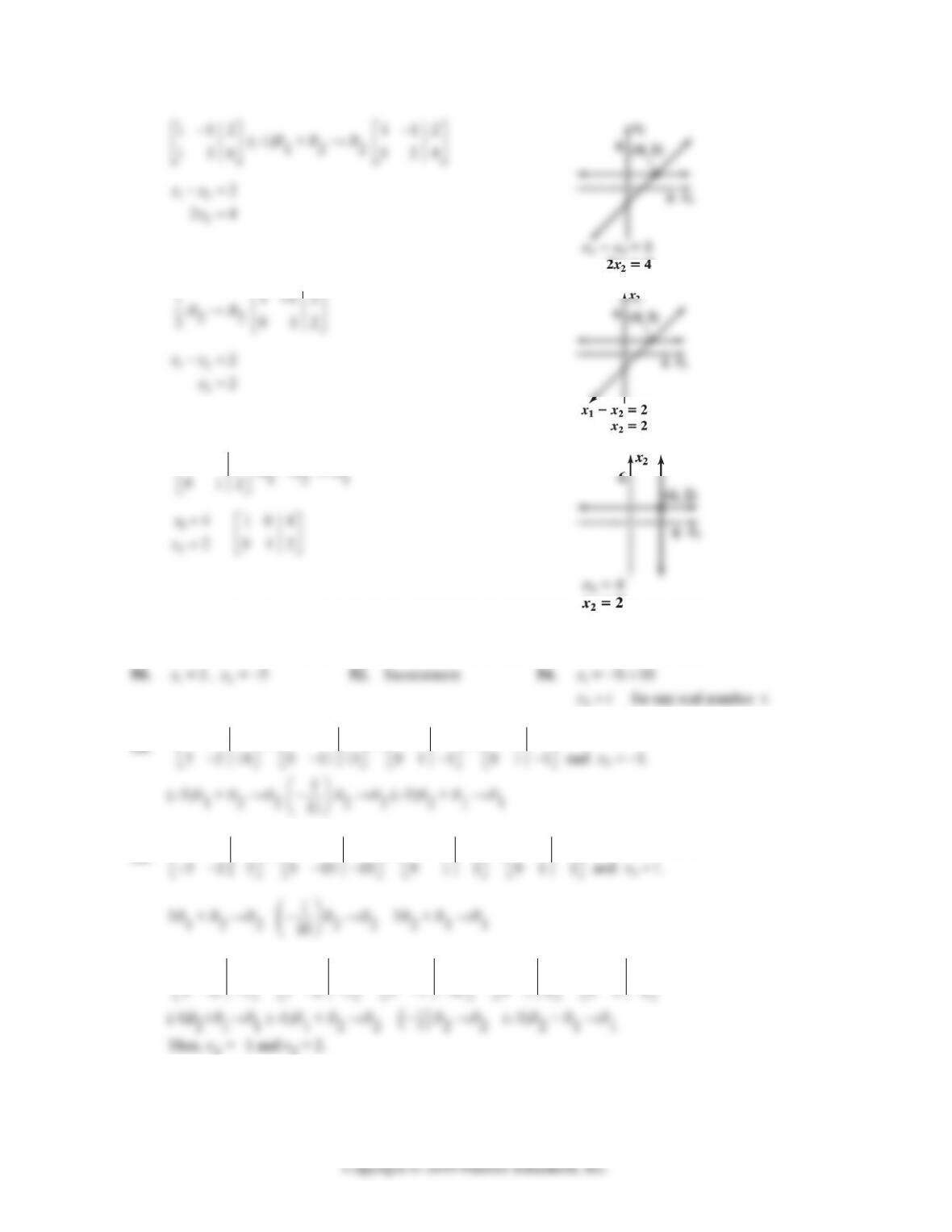
12
2
2
24
xx
x
2
2
2
x
104
012
NOTE: Solution: x1 = 4, x2 = 2. Each pair of lines has the same intersection point.
11
58. 135
~ 135
~ 135
~ 10 2
1
Thus, 2
x
10
60.
210
~ 135
~ 13 5
~ 135
~ 10 1
1
EXERCISE 4-2 4-13
3
2
11
3
2
11
64. 315
135
~
5
1
33
1
135
~
5
1
33
10 20
33
1
0
~
5
1
33
1
012
2
66. 242
~ 121
~ 121
68. 624
~ 312
70. 218
~
1
2
14
~
1
14
2
~
1
2
14
2
72. 244
~ 122
~ 122
4-14 CHAPTER 4: SYSTEMS OF LINEAR EQUATIONS; MATRICES
Copyright © 2019 Pearson Education, Inc.
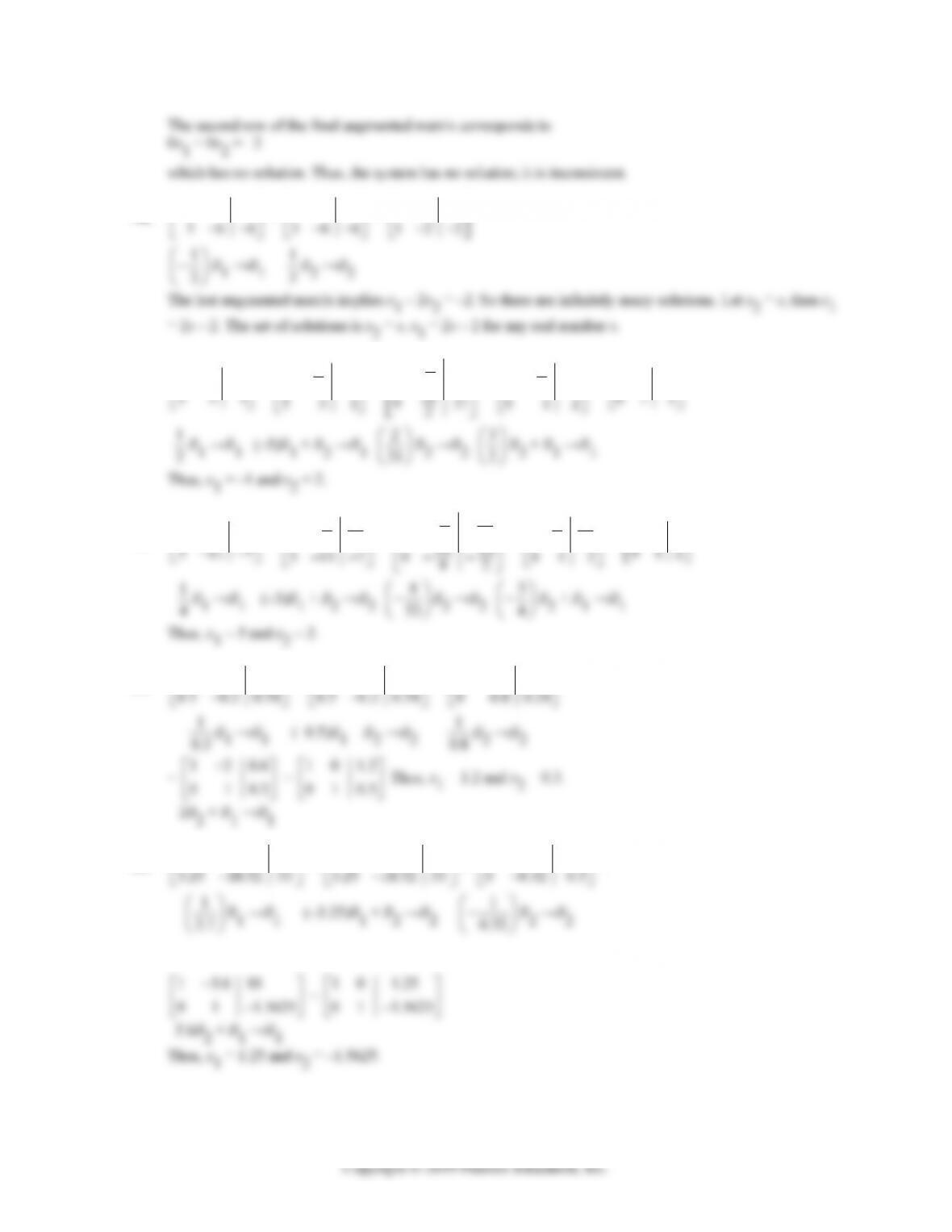
The second row of the final augmented matrix corresponds to
0x1 + 0x2 = –2
which has no solution. Thus, the system has no solution; it is inconsistent.
74. 244
~ 122
~ 122
76. 238
~
3
14
2
~
3
14
2
~
3
14
2
~ 10 1
78. 4326
~
313
142
~
313
142
~
313
142
~ 10 5
80. 0.3 0.6 0.18
~ 120.6
~ 120.6
82. 2.7 15.12 27
~ 15.610
~ 15.610
~
2.7
0.32
15.610
EXERCISE 4-3 4-15
84. 5.7 8.55 35.91
~ 11.56.3
~ 11.5 6.3
~
EXERCISE 4-3
418
34010
10. 01 3
12. 10 5
14.
510 5 15
02 2 7
16.
110 5 15
00 2 6
–1/2 R2 → R2
18.
10 5 15
01 2 7
4-16 CHAPTER 4: SYSTEMS OF LINEAR EQUATIONS; MATRICES
20. x1 = –2
x2 = 0
x3 = 1
22. x1 – 2x2 = –3 (1)
x3 = 5 (2)
24. x1 = 5
26. 10 1 4
0116
13
23
4
6
xx
xx
or 13
23
4
6
xx
xx
28. x1 – 2x3 + 3x4 = 4 (1)
x2 – x3 + 2x4 = –1 (2)
30. Problems 20 and 24. 32. Problems 22, 26, and 28.
34. False, for example:
100 2
000 1
36. True, if the system is consistent, then it either has infinitely many solutions or exactly one solution. If there
EXERCISE 4-3 4-17
Copyright © 2019 Pearson Education, Inc.
38. False. The system corresponding to the reduced form 10 18
0123
has infinitely many solutions.
40. 13 1
~ 13 1
~ 10 7
42. 111 8
(–3)R1 + R2 →R2 1118
1
0123
01 23
44.
10 4 0
01 3 1
~
10 4 0
01 3 1
~
104 0
010 4
~
100 4
010 4
2
46.
1264
0282
~
1264
0141
~
1264
0141
~
1026
01 4 1
48. The corresponding augmented matrix is:
35 1 7
11 1 1
~
1111
3517
~
1111
0244
~
1111
0122
4-18 CHAPTER 4: SYSTEMS OF LINEAR EQUATIONS; MATRICES
50. The corresponding augmented matrix is:
15
10
52. 24 610
33 3 6
~ 12 35
11 12
~ 1235
0123
~ 12 35
01 23
54.
210
327
~
1
10
2
327
~ 7
1
10
2
07
2
~
1
10
2
012
~
10 1
01 2
1
56.
37 111
12 1 3
~
7111
1333
12 1 3
Thus 123
000 4xxx
which is not possible; no solution.
EXERCISE 4-3 4-19
58.
23521
1152
21111
~
1 4 10 23
1152
03915
~
141023
051525
03 915
1
60. 39126
2684
~ 1342
2684
~ 1 342
0 000
4225
5
11
1224
5
11
122 4
11
64. (A)
10
01
ma
nb
,
10
011
ma
b
,
1
0000
mna
10 0
00 01
m
10
0000
mn
100
0001
m
66. 24548
~ 12335
~ 12 3 3 5
4-20 CHAPTER 4: SYSTEMS OF LINEAR EQUATIONS; MATRICES
Copyright © 2019 Pearson Education, Inc.
~
12 0 3 1
00 1 2 2
~ 120 3 1
001 2 2
124
34
Thus, 2 3 1
22
xxx
xx
(–1)R2→R2
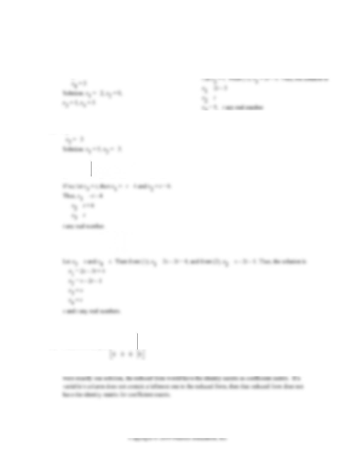
Letx2 = t, x4 = s, then x3 = –2s + 2 and x1 = –2t + 3s – 1.
Solution: x1 = –2t + 3s – 1; x2 = t; x3 = –2s + 2; x4 = s for t, s any real numbers.
68.
11 41 1.3
11 10 1.1
~
11411.3
02312.4
~
11411.3
31
01 1.2
22
2