CHAPTER 4 REVIEW 4-61
4. A = 53 102
48 130
, B =
32
04
5. (A) 12
13
1
2
x
x
= 4
2
x
x
(B)
53
11
1
2
x
x
+ 25
14
= 18
22
x
x
x
x
6. A + B = 12 21
= 33
7. B + D = 21
+ 1

4-62 CHAPTER 4: SYSTEMS OF LINEAR EQUATIONS; MATRICES
9. AB = 12
21
=
21
12 12
11
= 43
(4-4)
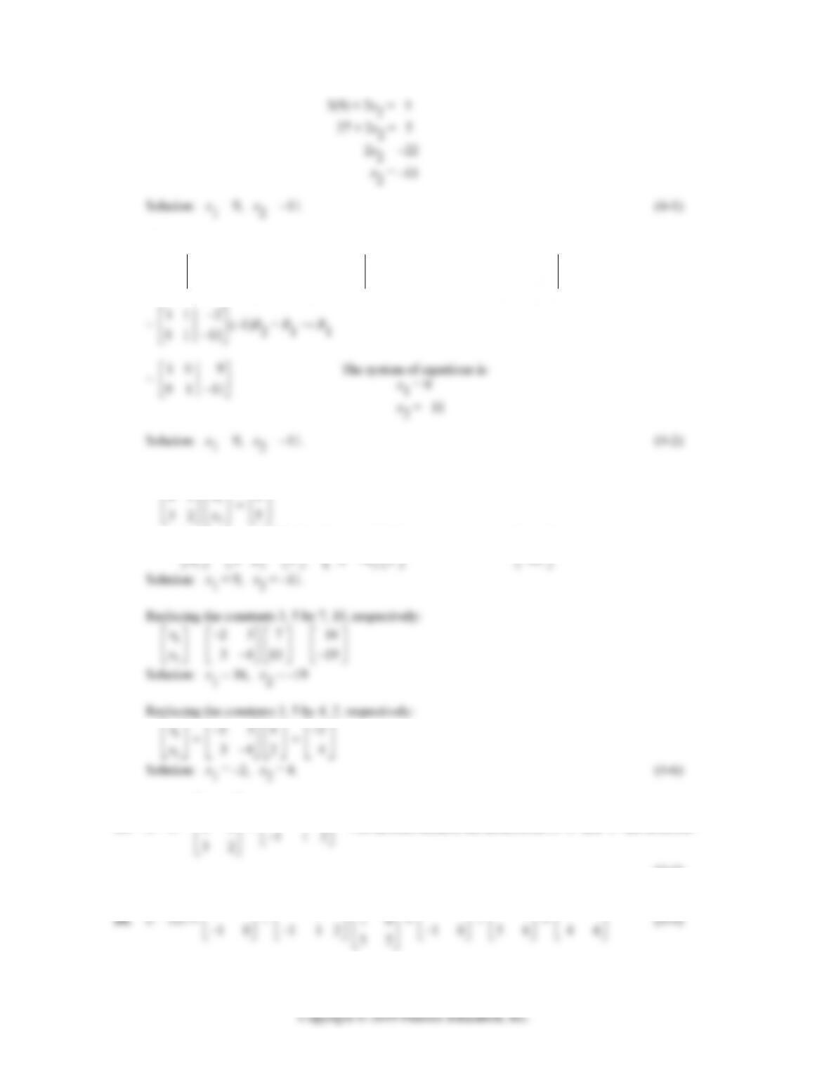
10. AC is not defined because the dimension of A is 2 × 2 and the dimension of C is 1 × 2. So, the number of
11. AD = 12
1
=
1
122
= 5
(4-4)
15. 4310
3201
(–1)R2 + R1 → R1 ~ 111 1
320 1
(–3)R1 + R2 → R2
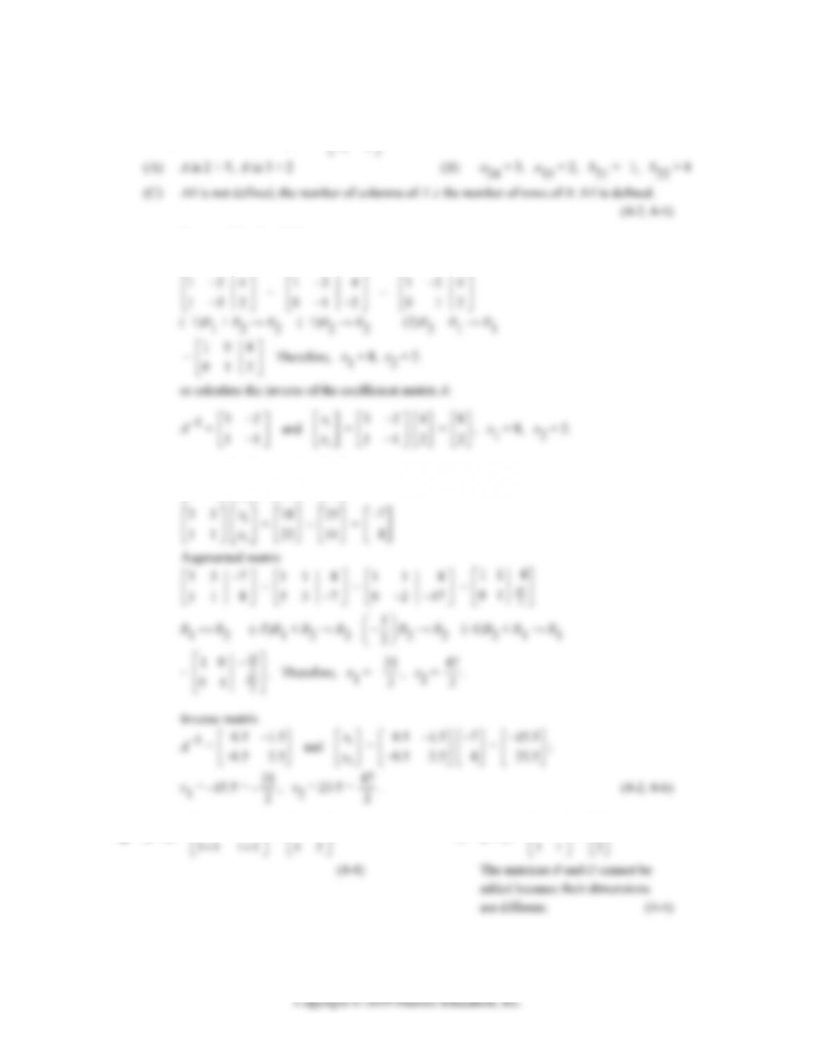
16. 4x1 + 3x2 = 3 (1) Multiply (1) by 2 and (2) by –3.

CHAPTER 4 REVIEW 4-63
17. The augmented matrix of the system is:
433
325
(–1)R2 + R1 → R1 ~
11 2
32 5
(–3)R1 + R2 → R2 ~ 112
0111
(–1)R2 → R2
18. The system of equations in matrix form is:
x
x
Thus, 1
x
x
= 43
–1 3
= 23
3
(by Problem 15) = 9
x
x
x
x
19. A + D =
22
10
+ 321
Not defined because the dimensions of A and D are different.
(4-4)
22
4-64 CHAPTER 4: SYSTEMS OF LINEAR EQUATIONS; MATRICES
21. From Problem 20, DA = 74
56
. Thus,
22. BC =
1
2
[2 1 3] =
213
426
(4-4)
23. CB = [2 1 3]
1
2
= [–2 + 2 + 9] = [9] (a 1 × 1 matrix) (4-4)
24. AD – BC
22
862
1
213
862
213
8(2) 6(1) 2(3)
25.
123 100
234010
~
12 3 100
012210
~
12 3 1 00
01 2 2 10

CHAPTER 4 REVIEW 4-65
Check:
51
22
2
123
100
26. (A) The augmented matrix corresponding to the given system is:
1231
1231
12 3 1
10 1 3
1013
100 2
(B) The augmented matrix corresponding to the given system is:
12 1 2
1212
1212
~
10512
01 3 7
(C) The augmented matrix corresponding to the given system is:
4-66 CHAPTER 4: SYSTEMS OF LINEAR EQUATIONS; MATRICES
Thus, x1 + 2x3 = 5
27. (A) The matrix equation for the given system is:
123
1
x
x
x
1
The inverse matrix of the coefficient matrix of the system, from Problem 25, is:
51
22
2
1
x
x
x
51
22
2
1
2
(B)
1
2
x
x
x
=
51
22
2
11 1
0
0
=
1
2
Solution: x1 = 1,
x2 = –2
(C)
1
2
x
x
x
=
51
22
2
11 1
3
4
=
1
2
Solution: x1 = –1,
x2 = 2,
28. 2x1 – 6x2 = 4
–x1 + kx2 = –2
29. M = 0.2 0.15
0.4 0.3
; I – M = 0.8 0.15
0.4 0.7
=
3
4
520
7
2
510
3
4
10
3
4
10
35
10
73
10
CHAPTER 4 REVIEW 4-67
The output matrix X is given by
X = (I – M)–1D = 1.4 0.3
30
= 48
A
30. T = 0.3 0.4
0.15 0.2
, D = 20
30
0.15 0.8
20 5
72
10
10
4
10
10
4
10
10
4
77
10
84
55
10
7
84
55
The output matrix X is given by
20 56
E
(4-7)
31. M = 0.45 0.65
; I – M = 0.55 0.65
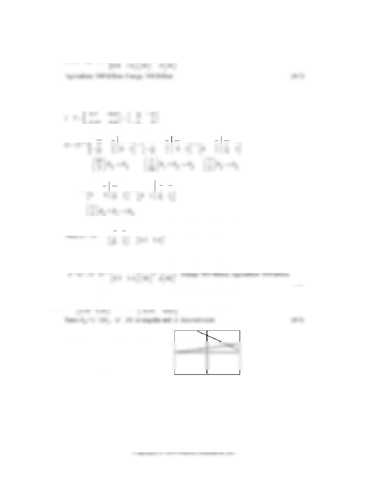
32. The graphs of the two equations are:
x ≈ 3.46, y ≈ 1.69 (4-1)
4-68 CHAPTER 4: SYSTEMS OF LINEAR EQUATIONS; MATRICES
33.
45 6100
45 4010
11 100 1
R1 ↔ R3 ~
11 100 1
45 4010
45 6100
12 2
13 3
(4)
(4)
RR R
RR R
~
10 9 0 1 5
01 8 0 1 4
31 1
(9)
8
RR R
RR R
~
91
10 10
82
10 10
100 5
010 4
0.9 0.1 5 4 5 6 1 0 0
34. The given system is equivalent to:
4x1 + 5x2 + 6x3 = 36,000
4x1 + 5x2 – 4x3 = 12,000
x1 + x2 + x3 = 7,000
In matrix form, this system is:
45 6
x
x
x
36,000
Thus,
1
x
x
x
45 6
–1 36,000
0.9 0.1 5
36,000
1, 400
35. First, multiply the first two equations of the system by 100. Then the augmented matrix of the resulting
system is:
45 636,000
11 1 7,000
1 1 1 7, 000
10 9 23,000
CHAPTER 4 REVIEW 4-69
10 9 23,000
(9)
RR R
100 1,400
1
1, 400
x
36. M =
0.2 0 0.4
0.1 0.3 0.1
=
12
55
3
11
10 10 10
0
and D =
40
20
42
0100
5
1
10 00
5
4R1 → R1 1
10 R1 + R2 → R2
5
1
24
10 00
5
1
24
10 00
5
1
24
10 0 0
5
1
24
10 0 0
5
1
24
10 0 0
13 7
2
10 5 10
100
13 7
2
10 5 10
1.3 0.4 0.7
4-70 CHAPTER 4: SYSTEMS OF LINEAR EQUATIONS; MATRICES
37. (A) The system has a unique solution.
38. (A) The system has a unique solution.
39. The third step in (A) is incorrect:
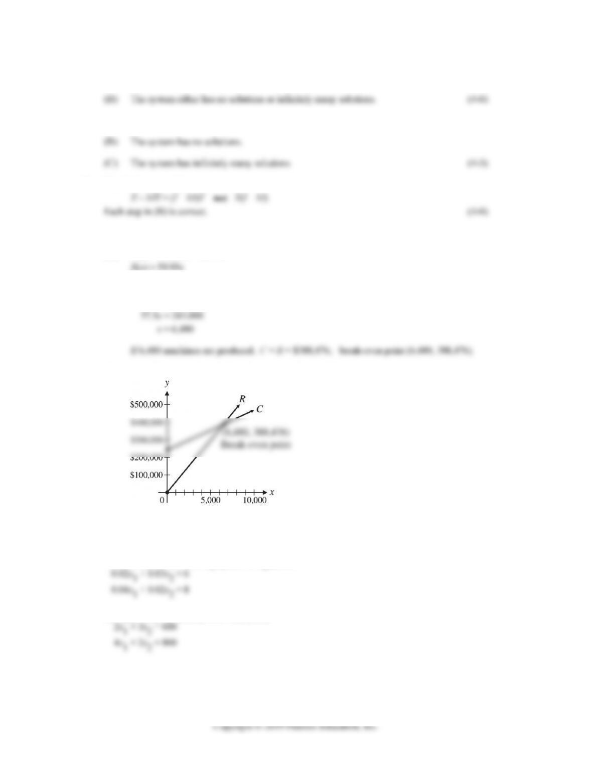
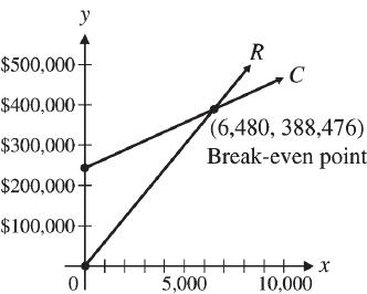
40. Let x = the number of machines produced.
(A) C(x) = 243,000 + 22.45x
(B) Set C(x) = R(x):
59.95x = 243,000 + 22.45x
(C) A profit occurs if x > 6,480; a loss occurs if x < 6,480
(4-1)
41. Let x1 = Number of tons of Voisey‘s Bay ore
x2 = number of tons of Hawk Ridge ore
Then, we have the following system of equations
Multiply each equation by 100. This yields
The augmented matrix corresponding to this system is:

CHAPTER 4 REVIEW 4-71
42. (A) The matrix equation for Problem 41 is:
x
x
50R1 → R1 (–0.04)R1 + R2 → R2 1
0.04
R2 → R2
11.550 0
Thus, the inverse of the coefficient matrix is:
25 37.5
50 25
x
x
x
x
7.5
(4-6)
43. (A) Let x1 = number of 3,000 cubic foot hoppers
Then
3,000x1 + 4,500x2 + 6,000x3 = 108,000
4-72 CHAPTER 4: SYSTEMS OF LINEAR EQUATIONS; MATRICES
The augmented matrix for this system is:
Now
The corresponding system of equations is:
x1 – x3 = –12
(B) Cost: C(t) = 180(t – 12) + 225(32 – 2t) + 325(t)
C(12) = 225(8) + 325(12) = $5,700
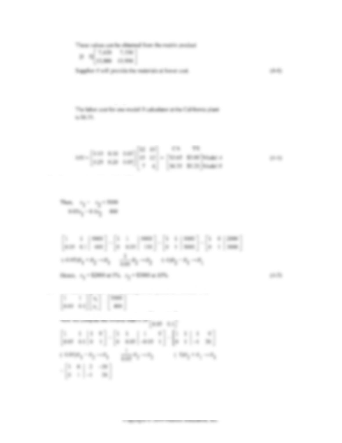
44. (A) The elements of MN give the cost of materials for each alloy from each supplier. The product
(B) MN =
0.75 0.70
4,800 600 300 6.50 6.70
(C) The total costs of materials from Supplier A is:
$7,620 + $13,880 = $21,500

CHAPTER 4 REVIEW 4-73
45. (A) [0.25 0.20 0.05]
12
15
7
= 6.35
The elements of MN give the total labor costs for each calculator at each plant. The product NM is
also defined, but does not have an interpretation in the context of this problem.
46. Let x1 = amount invested at 5%
and x2 = amount invested at 10%.
The augmented matrix for the system given above is:
47. The matrix equation corresponding to the system in Problem 46 is:
11
4-74 CHAPTER 4: SYSTEMS OF LINEAR EQUATIONS; MATRICES
Thus, the inverse of the coefficient matrix is 220
, and
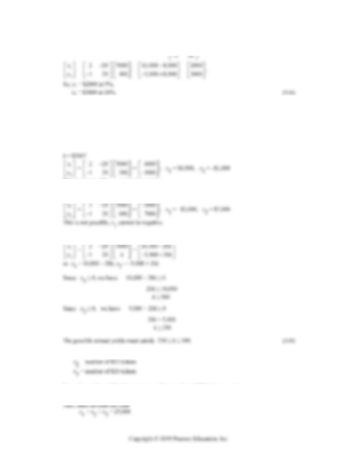
48. From Problem 46, the system of equations is:
x1 + x2 = 5000
0.05x1 + 0.1x2 = k (annual return)
From Problem 47, the inverse of the coefficient matrix A is: A–1 = 220
120
This is not possible, x2 cannot be negative.
k = $600?
Fix a return k. Then
49. Let x1 = number of $8 tickets
Since the number of $8 tickets must equal the number of $20 tickets, we have
x1 = x3 or x1 – x3 = 0

CHAPTER 4 REVIEW 4-75
Finally, the return is
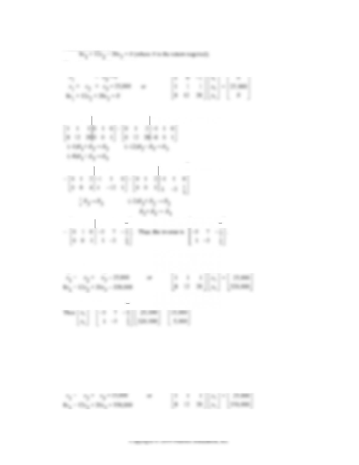
Thus, the system of equations is:
x
x
x
First, we compute the inverse of the coefficient matrix
10 1100
10 1100
10 11 0 0
10 11 0 0
1
4
100 2 3
1
4
23
Concert 1:
x1 – x3 = 0
10 1
1
x
x
x
0
1
x
x
x
1
4
23
0
5,000
and x1 = 5,000 $8 tickets
x2 = 15,000 $12 tickets
x3 = 5,000 $20 tickets
Concert 2:
x1 – x3 = 0
10 1
1
x
x
0
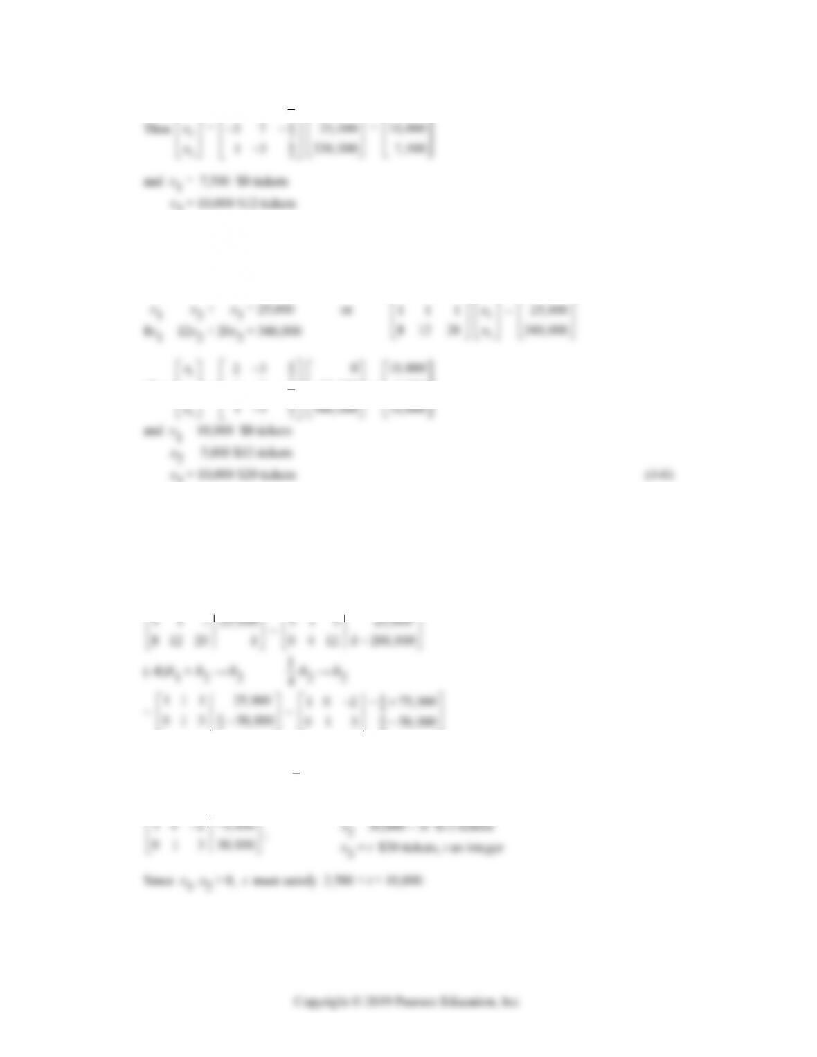
4-76 CHAPTER 4: SYSTEMS OF LINEAR EQUATIONS; MATRICES
1
x
x
x
1
4
23
0
7,500
x3 = 7,500 $20 tickets
Concert 3:
x1 – x3 = 0
10 1
1
x
x
x
0
Thus
2
x
x
x
=
1
2
1
37
25,000
=
5, 000
50. From Problem 49, if it is not required to have an equal number of $8 tickets and $12 tickets, then the new
mathematical model is:
x1 + x2 + x3 = 25,000
8x1 + 12x2 + 20x3 = k (return requested)
The augmented matrix is:
4
4
(–1)R2 + R1 → R1
Concert 1: k = $320,000; 1
4k = 80,000
x1 = 2t – 5,000 $8 tickets

01 332,500
;
x3 = t $20 tickets, t an integer
Since x1, x2 ≥ 0, t must satisfy 3,750 ≤ t ≤ 10,833.
Concert 3: k = $340,000; 1
51. The technology matrix is
Agriculture Fabrication
01
0.20 0.40
0.20 0.60
55
Next, we calculate the inverse of I – M
71
~
31
24
10
Thus, (I – M)–1 =
31
24
.
(A) Let D = 50
. Then X =
31
24
50
= 75 5
= 80
4-78 CHAPTER 4: SYSTEMS OF LINEAR EQUATIONS; MATRICES
52. First we find the inverse of B =
110
10 1
111
.
110100
110100
11 0 1 00
~
10 1 0 10
011110
00 1 1 01
~
101111
010 0 1 1
001 1 0 1
Thus, B–1 =
111
011
10 1
.
(–1)R3 + R1 → R1
53. (A) 1st & Elm: x1 + x4 = 1300
2nd & Elm: x1 – x2 = 400
(B) The augmented matrix for the system in part (A) is:
1 0 0 1 1300
1 0 0 1 1300
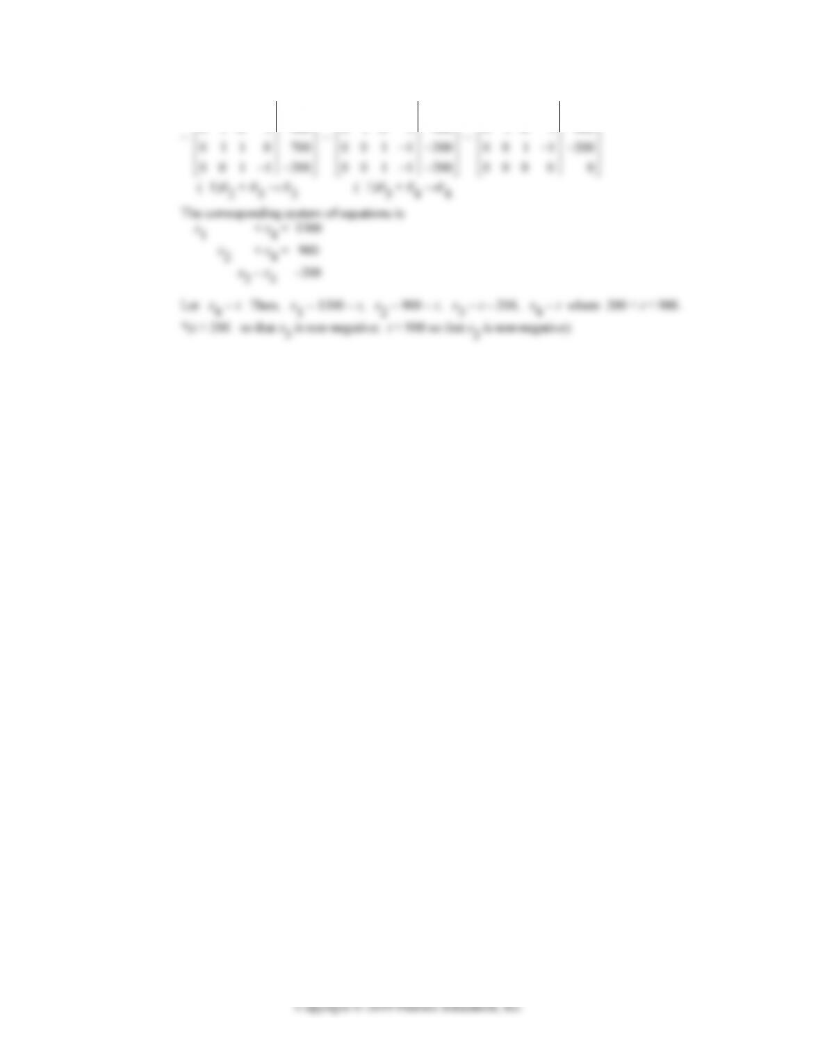

CHAPTER 4 REVIEW 4-79
1 0 0 1 1300
010 1 900
1 0 0 1 1300
010 1 900
1 0 0 1 1300
010 1 900
(C) maximum: 900, minimum: 200
(D) Elm St.: x1 = 800; 2nd St.: x2 = 400; Oak St.: x3 = 300. (4-3)