Markov Processes
Chapter 4
Decision Analysis
Learning Objectives
1. Learn how to describe a problem situation in terms of decisions to be made, chance events and
consequences.
5. Be able to determine the potential value of additional information.
6. Learn how new information and revised probability values can be used in the decision analysis
approach to problem solving.
7. Understand what a decision strategy is.
8. Learn how to evaluate the contribution and efficiency of additional decision making information.
9. Be able to use a Bayesian approach to compute revised probabilities.
10. Be able to use TreePlan software for decision analysis problems.
decision alternatives
decision strategy
chance events
risk profile
states of nature
sensitivity analysis
influence diagram
prior probabilities
payoff table
posterior probabilities
decision tree
expected value of sample information (EVSI)
optimistic approach
efficiency of sample information
conservative approach
Bayesian revision
minimax regret approach
opportunity loss or regret
expected value approach
expected value of perfect information (EVPI)
Chapter 17
Solutions:
1. a.
b.
Decision
Maximum Profit
Minimum Profit
d1
250
25
d2
100
75
Optimistic approach: select d1
Conservative approach: select d2
0
150
2. a.
Decision
Maximum Profit
Minimum Profit
d1
14
5
d2
11
7
d3
11
9
d4
13
8
Optimistic approach: select d1
s1
s3
s2
d1
250
100
25

Markov Processes
Regret or Opportunity Loss Table with the Maximum Regret
s1
s2
s3
s4
Maximum Regret
d1
0
1
1
8
8
d2
3
0
3
6
6
d3
5
0
1
2
5
d4
6
0
0
0
6
Minimax regret approach: select d3
b. The choice of which approach to use is up to the decision maker. Since different approaches can
result in different recommendations, the most appropriate approach should be selected before
analyzing the problem.
c.
Decision
Minimum Cost
Maximum Cost
d1
5
14
d2
7
11
d3
9
11
d4
8
13
s1
s2
s3
s4
Maximum Regret
d1
6
0
2
0
6
d2
3
1
0
2
3
d3
1
1
2
6
6
d4
0
1
3
8
8
Minimax regret approach: select d2
3. a. The decision to be made is to choose the best plant size. There are 2 alternatives to choose from: a
small plant or a large plant.
b. Influence Diagram:
Plant
Size
Market
Demand
Chapter 17
c.
d.
Decision
Maximum Profit
Minimum Profit
Maximum Regret
Small
200
150
300
Large
500
50
100
Optimistic approach: select Large plant
Conservative approach: select Small plant
Minimax regret approach: select Large plant
4. a. The decision faced by Amy is to select the best lease option from three alternatives (Hepburn Honda,
Midtown Motors, and Hopkins Automotive). The chance event is the number of miles Amy will
drive.
for the Midtown Motors lease option:
36000 miles (12000 miles for 3 years): 36($310) + $0.20*max(36000 – 45000,0) = $11,160.00
45000 miles (15000 miles for 3 years): 36($310) + $0.20*max(45000 – 45000,0) = $11,160.00
54000 miles (18000 miles for 3 years): 36($310) + $0.20*max(54000 – 45000,0) = $12,960.00
Small
Low
Medium
High
150
200
200
Markov Processes
So the payoff table for Amy’s problem is:
Actual Miles Driven Annually
Dealer 12000 15000 18000
Hepburn Honda $10,764 $12,114 $13,464
c. The minimum and maximum payoffs for each of Amy’s three alternatives are:
Dealer Minimum Cost Maximum Cost
Hepburn Honda $10,764 $13,464
Midtown Motors $11,160 $12,960
Hopkins Automotive $11,700 $11,700
Thus:
The optimistic approach results in selection of the Hepburn Automotive lease option (which has the
smallest minimum cost of the three alternatives – $10,764).
The regret table for this problem is
State of Nature (Actual Miles Driven Annually)
Decision Alternative 12000 15000 18000 Maximum Regret
Hepburn Honda $0 $954 $1,764 $1,764
d. We first find the expected value for the payoffs associated with each of Amy’s three alternatives:
EV(Hepburn Honda) = 0.5($10,764) + 0.4($12,114) + 0.1($13,464) = $11,574
EV(Midtown Motors) = 0.5($11,160) + 0.4($11,160) + 0.1($12,960) = $11,340
Chapter 17
e. The risk profile for the decision to lease from Midtown Motors is:
Note that although we have three chance outcomes (drive 12000 miles annually, drive 15000 miles
annually, and drive 18000 miles annually), we only have two unique costs on this graph. This is
because for this decision alternative (lease from Midtown Motors) there are only two unique payoffs
associated with the three chance outcomes – the payoff (cost) associated with the Midtown Motors
lease is the same for two of the chance outcomes (whether Amy drives 12000 miles or 15000 miles
annually, her payoff is $11,160).
f. We first find the expected value for the payoffs associated with each of Amy’s three alternatives:
EV(Hepburn Honda) = 0.3($10,764) + 0.4($12,114) + 0.3($13,464) = $12,114
Markov Processes
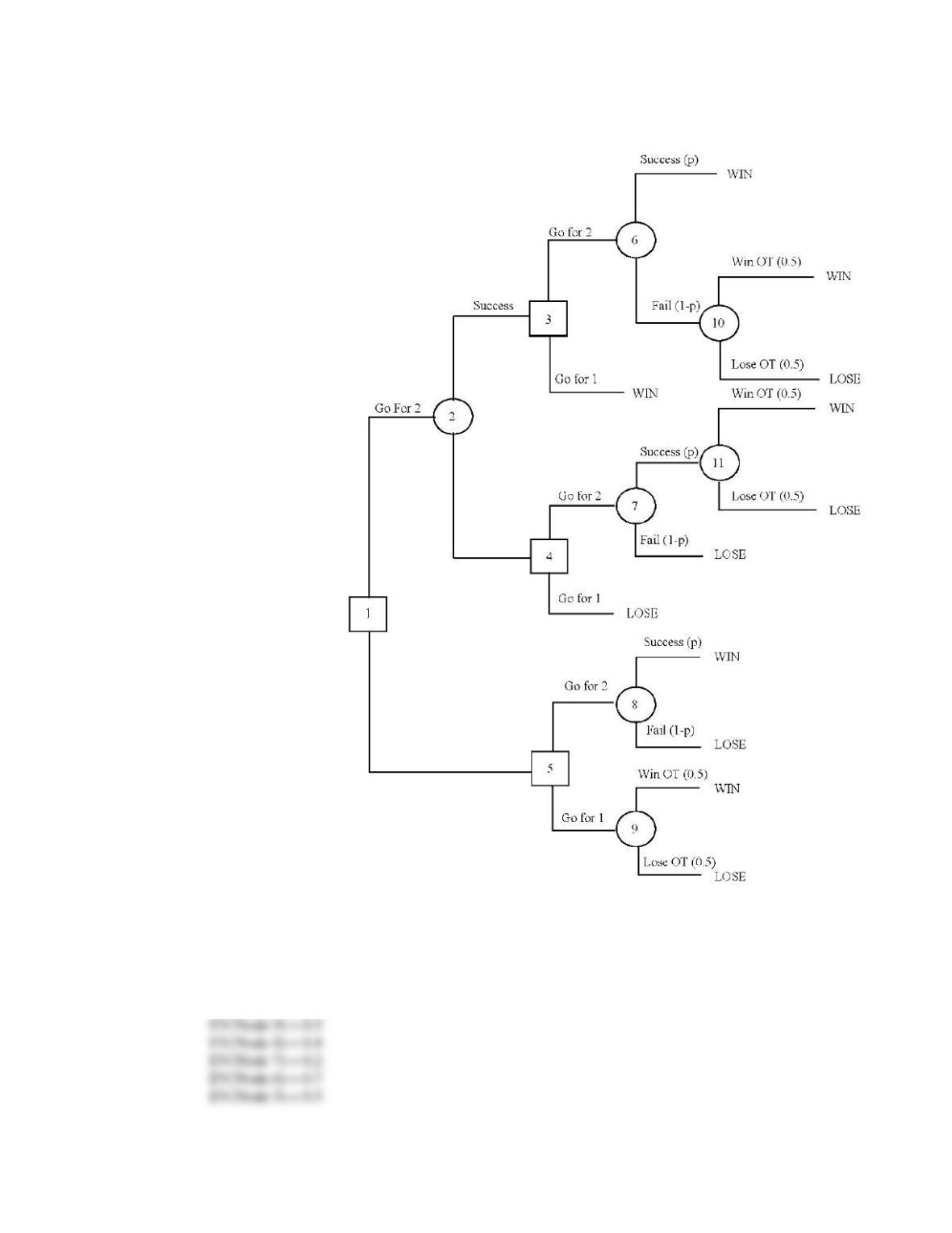
5. a.
b. Let p = 0.4 in decision tree, the value for terminal node= Win is 1, and the value for terminal node =
LOSE is 0. Then
EV(Node 11) = 0.5
EV(Node 10) = 0.5
Chapter 17
EV(Node 4) = 0.2
6. a. EV(C) = 0.2(10) + 0.5(2) + 0.3(-4) = 1.8
EV(F) = 0.2(8) + 0.5(5) + 0.3(-3) = 3.2
EV(M) = 0.2(6) + 0.5(4) + 0.3(-2) = 2.6
EV(P) = 0.2(6) + 0.5(5) + 0.3(-1) = 3.4
Pharmaceuticals recommended 3.4%
b. Using probabilities 0.4, 0.4, 0.2.
7. a. EV(own staff) = 0.2(650) + 0.5(650) + 0.3(600) = 635
EV(outside vendor) = 0.2(900) + 0.5(600) + 0.3(300) = 570
EV(combination) = 0.2(800) + 0.5(650) + 0.3(500) = 635
The optimal decision is to hire an outside vendor with an expected annual cost of $570,000.
b. The risk profile in tabular form is shown.
Cost
Probability
300
0.3
600
0.5
900
0.2
1.0
A graphical representation of the risk profile is also shown:
0.3
0.4
0.5
Markov Processes
8. a. EV(d1) = p(10) + (1 – p) (1) = 9p + 1
EV(d2) = p(4) + (1 – p) (3) = 1p + 3
9p + 1 = 1p + 3 and hence p = .25
d2 is optimal for p 0.25; d1 is optimal for p 0.25.
b. The best decision is d2 since p = 0.20 < 0.25.
EV(d1) = 0.2(10) + 0.8(1) = 2.8
EV(d2) = 0.2(4) + 0.8(3) = 3.2
As long as the payoff for s1 is 2, then d2 will be optimal.
9. a. The decision to be made is to choose the type of service to provide. The chance event is the level of
demand for the Myrtle Air service. The consequence is the amount of quarterly profit. There are
two decision alternatives (full price and discount service). There are two outcomes for the chance
event (strong demand and weak demand).
b.
Type of Service
Maximum Profit
Minimum Profit
10
Chapter 17
Optimistic Approach: Full price service
High Demand
Low Demand
Maximum Regret
Full Service
0
810
810
Discount Service
290
0
290
Minimax Regret Approach: Discount service
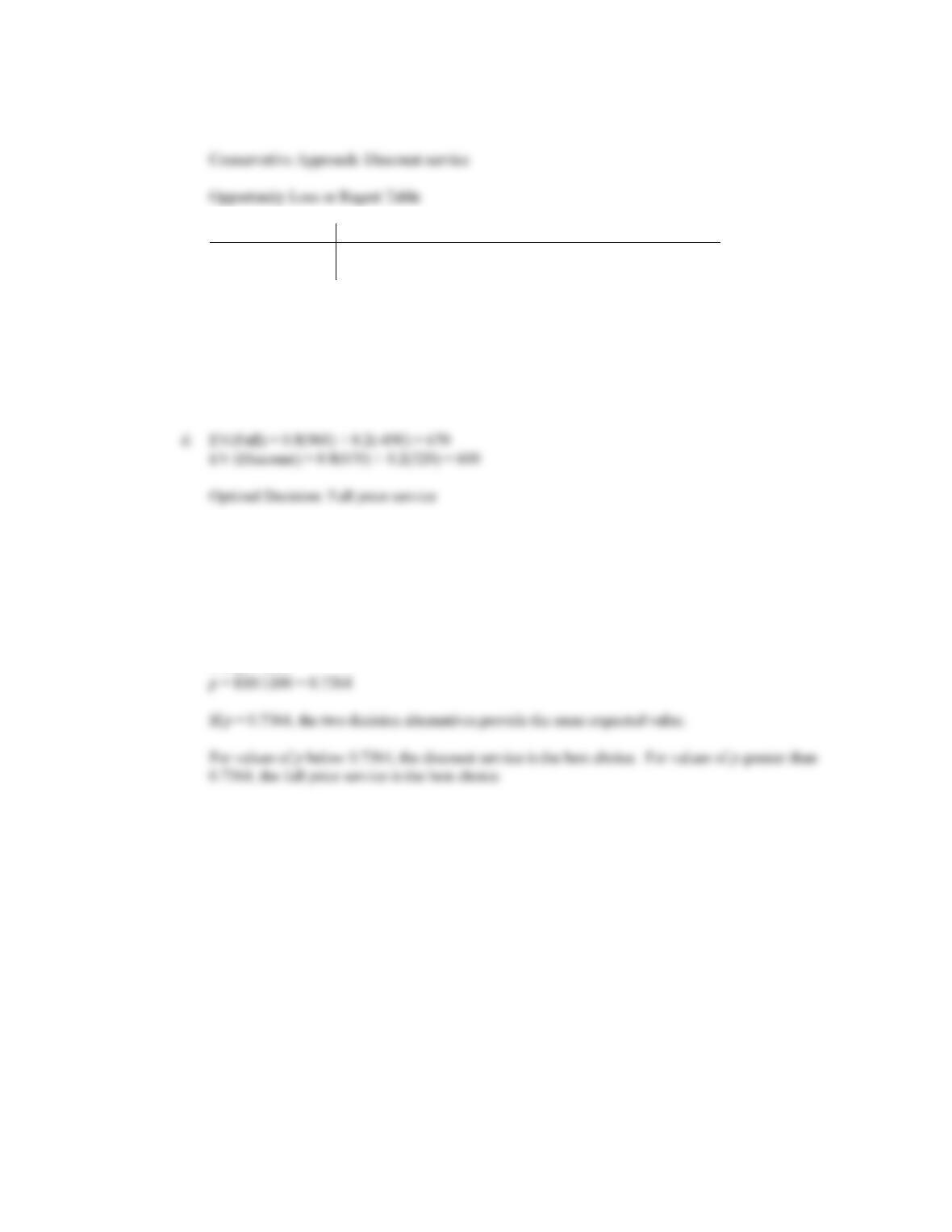
c. EV(Full) = 0.7(960) + 0.3(-490) = 525
EV (Discount) = 0.7(670) + 0.3(320) = 565
Optimal Decision: Discount service
e. Let p = probability of strong demand
EV(Full) = p(960) + (1- p)(–490) = 1450p – 490
EV (Discount) = p(670) + (1- p)(320) = 350p + 320
EV (Full) = EV(Discount)
1450p – 490 = 350p + 320
Markov Processes
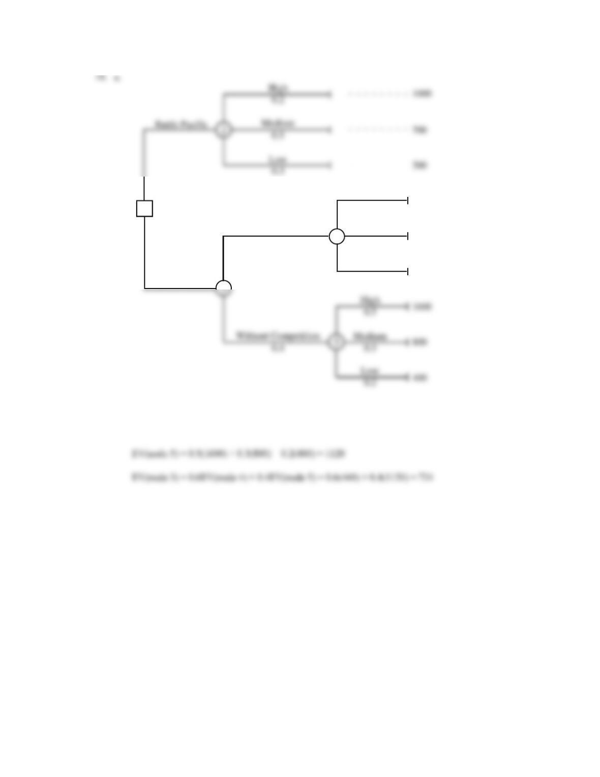
b. EV(node 2) = 0.2(1000) + 0.5(700) + 0.3(300) = 640
EV(node 4) = 0.3(800) + 0.4(400) + 0.3(200) = 460
Space Pirates is recommended. Expected value of $724,000 is $84,000 better than Battle Pacific.
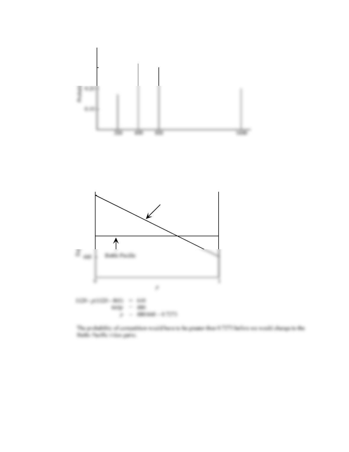
c. Risk Profile for Space Pirates
Outcome:
1600 (0.4)(0.5) = 0.20
800 (0.6)(0.3) + (0.4)(0.3) = 0.30
400 (0.6)(0.4) + (0.4)(0.2) = 0.32
200 (0.6)(0.3) = 0.18
1
200
400
800
High
Medium
Low
0.3
0.4
0.3
4
With Competition
0.6
Space Pirates
Chapter 17
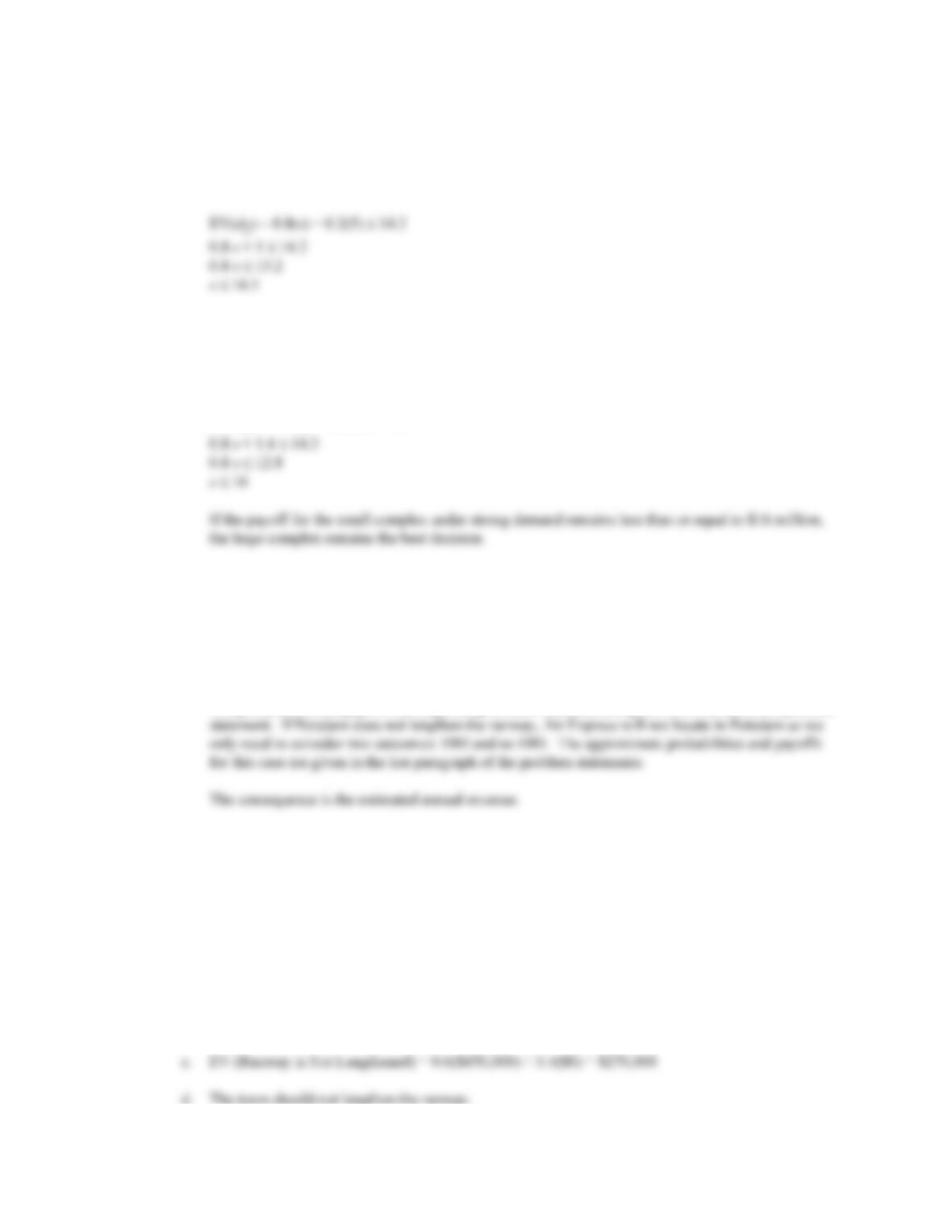
d. Let p = probability of competition
p = 0 EV(node 5) = 1120
p = 1 EV(node 4) = 460
0.30
Profit ($ thousands)
1120
640
Space Pirates
Markov Processes
11. a. Currently, the large complex decision is optimal with EV(d3) = 0.8(20) + 0.2(-9) = 14.2. In order
for d3 to remain optimal, the expected value of d2 must be less than or equal to 14.2.
Let s = payoff under strong demand
Thus, if the payoff for the medium complex under strong demand remains less than or equal to $16.5
million, the large complex remains the best decision.
b. A similar analysis is applicable for d1
EV(d1) = 0.8(s) + 0.2(7) 14.2
12. a. There is only one decision to be made: whether or not to lengthen the runway. There are only two
decision alternatives. The chance event represents the choices made by Air Express and DRI
concerning whether they locate in Potsdam. Even though these are decisions for Air Express and
DRI, they are chance events for Potsdam.
The payoffs and probabilities for the chance event depend on the decision alternative chosen. If
Potsdam lengthens the runway, there are four outcomes (both, Air Express only, DRI only, neither).
The probabilities and payoffs corresponding to these outcomes are given in the tables of the problem
b. Runway is Lengthened
New
Air Express Center
New
DRI Plant
Probability
Annual Revenue
Yes
Yes
0.3
$600,000
Yes
No
0.1
$150,000
No
Yes
0.4
$250,000
No
No
0.2
-$200,000
EV (Runway is Lengthened) = 0.3($600,000) + 0.1($150,000) + 0.4($250,000) – 0.2($200,000)
= $255,000
Chapter 17
e. EV (Runway is Lengthened) = 0.4(600,000) + 0.1($150,000) + 0.3($250,000) – 0.2(200,000)
= $290,000
The revised probabilities would lead to the decision to lengthen the runway.
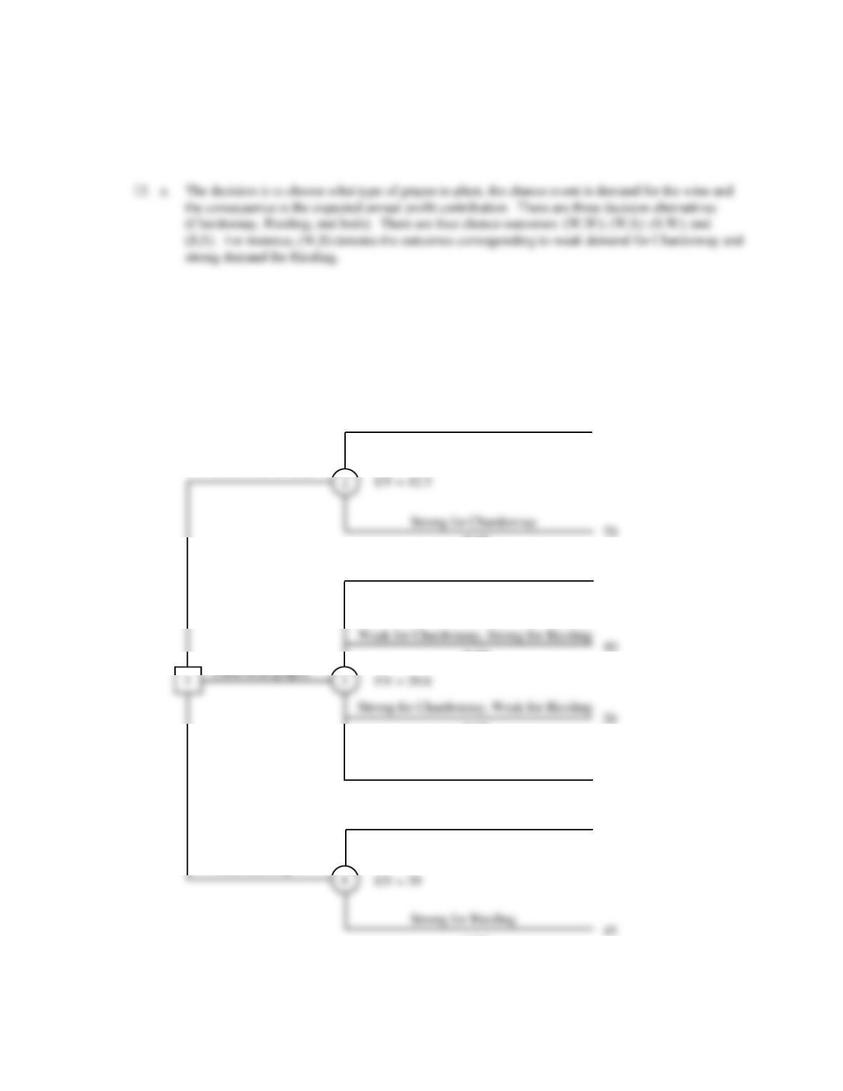
b. In constructing a decision tree, it is only necessary to show two branches when only a single grape is
planted. But, the branch probabilities in these cases are the sum of two probabilities. For example,
the probability that demand for Chardonnay is strong is given by:
P (Strong demand for Chardonnay) = P(S,W) + P(S,S)
= 0.25 + 0.20
= 0.45
Plant Chardonnay
Plant Riesling
Weak for Chardonnay
0.55
0.45
Weak for Chardonnay, Weak for Riesling
0.05
0.50
0.25
Strong for Chardonnay, Strong for Riesling
0.20
Weak for Riesling
0.30
0.70
20
22
60
25