CHAPTER 4
Regression Models
TEACHING SUGGESTIONS
Teaching Suggestion 4.1: Which Is the Independent Variable?
We find that students are often confused about which variable is independent and which is de-
pendent in a regression model. For example, in Triple A’s problem, clarify which variable is X
Teaching Suggestion 4.2: Statistical Correlation Does Not Always Mean Causality.
Students should understand that a high r2 doesn’t always mean one variable will be a good pre-
Teaching Suggestion 4.3: Give students a set of data and have them plot the data and manually
draw a line through the data. A discussion of which line is “best” can help them appreciate the
least squares criterion.
Teaching Suggestion 4.4: Select some randomly generated values for X and Y (you can use ran-
dom numbers from the random number table in Chapter 15 or use the RAND function in Excel).
Develop a regression line using Excel and discuss the coefficient of determination and the F-test.
Students will see that a regression line can always be developed, but it may not necessarily be
useful.
Teaching Suggestion 4.5: A discussion of the long formulas and short-cut formulas that are pro-
vided in the appendix is helpful. The long formulas provide students with a better understanding
ALTERNATIVE EXAMPLES
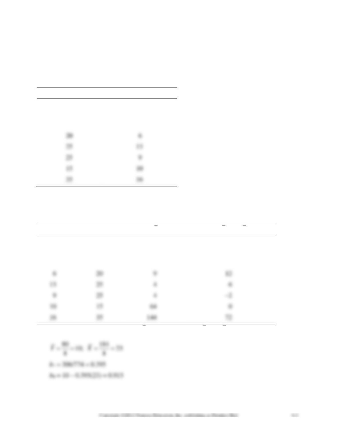
Alternative Example 4.1: The sales manager of a large apartment rental complex feels the de-
mand for apartments may be related to the number of newspaper ads placed during the previous
month. She has collected the data shown in the accompanying table.
Ads purchased, (X)
Apartments leased, (Y)
15
6
9
4
40
16
25
13
25
9
15
10
35
16
We can find a mathematical equation by using the least squares regression approach.
(Note: Round-off error may cause this to be slightly different from a calculator solution.)
Leases, Y
Ads, X
(X –
X
)2
(X –
X
)(Y –
Y
)
6
15
64
32
4
9
196
84
16
40
289
102
6
20
9
12
13
25
4
6
9
25
4
10
15
64
0
Y = 80
X = 184
(X –
X
)2 = 774
(X –
X
)(Y –
Y
) = 306
The estimated regression equation is
ˆ
Y
= 0.915 + 0.395X
or
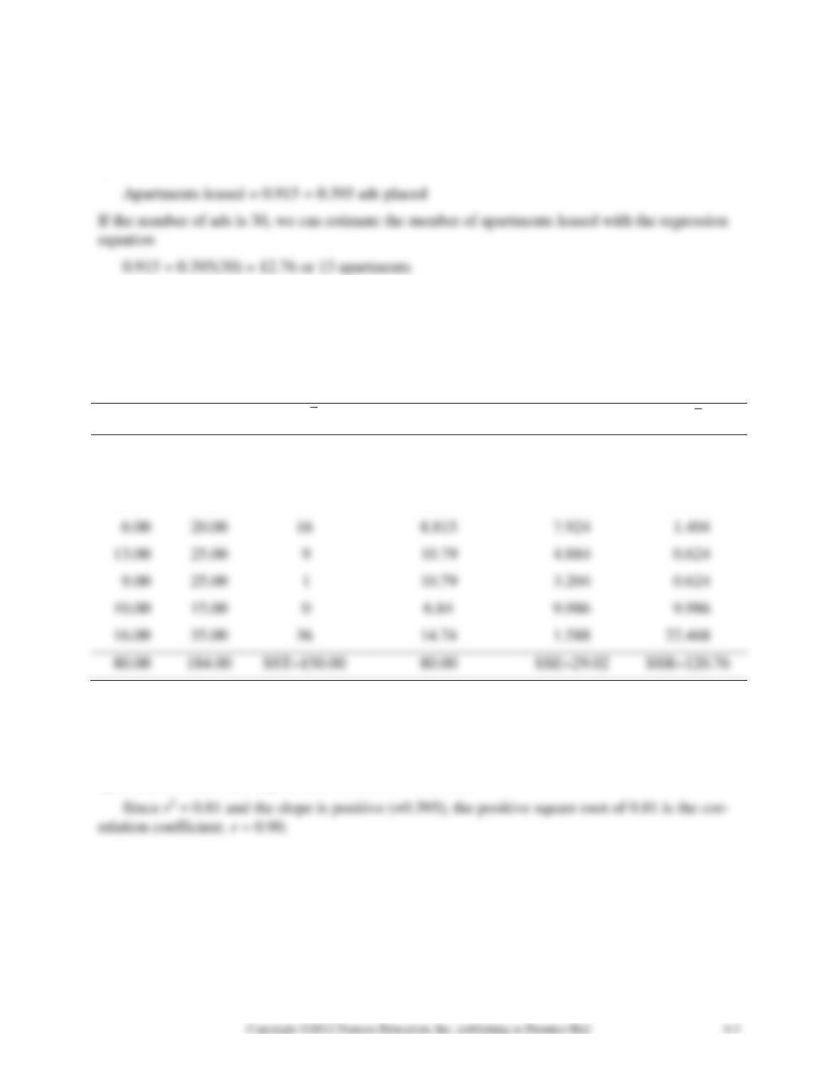
Alternative Example 4.2: Given the data on ads and apartment rentals in Alternative Example
4.1, find the coefficient of determination. The following have been computed in the table that
follows:
SST = 150; SSE = 29.02; SSR = 120.76
(Note: Round-off error may cause this to be slightly different from a computer solution.)
Y
X
(Y –
Y
)2
ˆ
Y
= 0.915 + 0.395X
(Y –
ˆ
Y
)2
(
ˆ
Y
–
Y
)2
6.00
15.00
16
6.84
0.706
9.986
4.00
9.00
36
4.47
0.221
30.581
16.00
40.00
36
16.715
0.511
45.091
6.00
20.00
16
7.924
1.404
13.00
25.00
4.884
0.624
9.00
25.00
3.204
0.624
10.00
15.00
6.84
9.986
9.986
16.00
35.00
36
1.588
22.468
80.00
SSE=29.02
From this the coefficient of determination is
r2 = SSR/SST = 120.76/150 = 0.81
Alternative Example 4.3: For Alternative Examples 4.1 and 4.2, dealing with ads, X, and
apartments leased, Y, compute the correlation coefficient.
SOLUTIONS TO DISCUSSION QUESTIONS AND PROBLEMS
4-2. Dummy variables are used when a qualitative factor such as the gender of an individual
(male or female) is to be included in the model. Usually this is given a value of 1 when the con-
4-3. The coefficient of determination (r2) is the square of the coefficient of correlation (r). Both
4-4. A scatter diagram is a plot of the data. This graphical image helps to determine if a linear
relationship is present, or if another type of relationship would be more appropriate.
4-5. The adjusted r2 value is used to help determine if a new variable should be added to a re-
gression model. Generally, if the adjusted r2 value increases when a new variable is added to a
4-6. The F-test is used to determine if the overall regression model is helpful in predicting the
value of the independent variable (Y). If the F-value is large and the p-value or significance level
4-8. When the residuals (errors) are plotted after a regression line is found, the errors should be
random and should not show any significant pattern. If a pattern does exist, then the assumptions
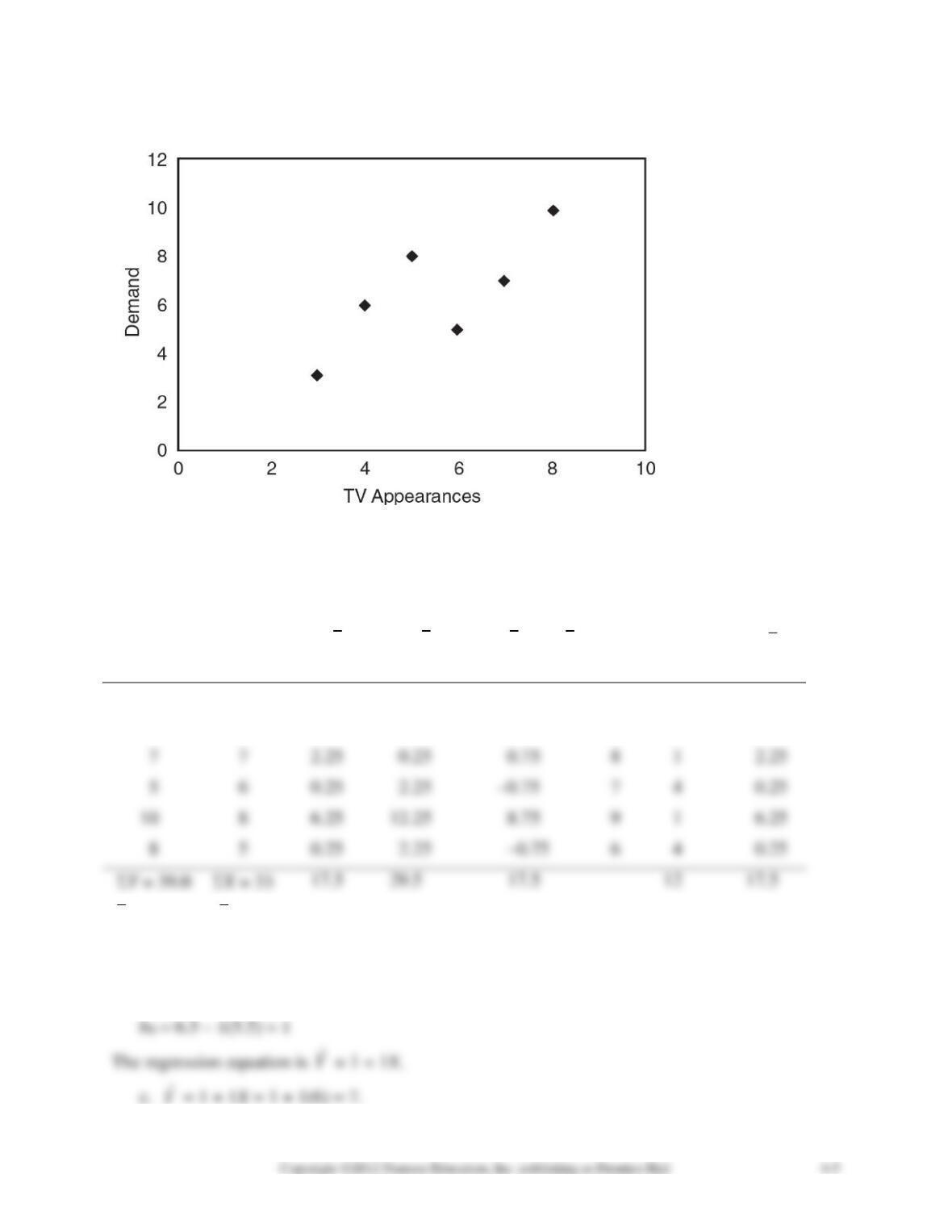
4-10. a.
4-10. b.
Demand = Y TV Appearances = X
Y
X
(X –
X
)2
(Y –
Y
)2
(X –
X
)(Y –
Y
)
ˆ
Y
(Y –
ˆ
Y
)2
(
ˆ
Y
–
Y
)2
3
3
6.25
12.25
8.75
4
1
6.25
6
4
2.25
0.25
0.75
5
1
2.25
7
7
2.25
0.25
0.75
8
1
2.25
5
6
0.25
2.25
7
4
0.25
10
8
6.25
12.25
8.75
9
1
6.25
8
5
0.25
2.25
6
4
0.25
Y
= 6.5
X
= 5.5
SST
SSE
SSR
SST = 29.5; SSE = 12; SSR = 17.5
b1 = 17.5/17.5 = 1
4-11. See the table for the solution to problem 4-10 to obtain some of these numbers.
MSE = SSE/(n – k – 1) = 12/(6 – 1 – 1) = 3
F0.05, 1, 4 = 7.71
Do not reject H0 since 5.83 7.71. Therefore, we cannot conclude there is a statistically signifi-
cant relationship at the 0.05 level.
4-12. Using Excel, the regression equation is
ˆ
Y
= 1 + 1X. F = 5.83, the significance level is
0.073. This is significant at the 0.10 level (0.073 0.10), but it is not significant at the 0.05 level.
4-13.
Fin. Ave
Test 1
(Y)
(X)
(X –
X
)2
(Y –
Y
)2
(X –
X
)(Y –
Y
)
Y
(Y –
ˆ
Y
)2
(
ˆ
Y
–
Y
)2
93
98
285.235
196
236.444
91.5
2.264
156.135
78
77
16.901
1
4.111
76
4.168
9.252
84
88
47.457
25
34.444
84.1
0.009
25.977
73
80
1.235
36
6.667
78.2
26.811
0.676
84
96
221.679
25
90
36.188
121.345
64
61
404.457
225
64.1
0.015
221.396
64
66
228.346
225
67.8
14.592
124.994
76
69
146.679
9
35.528
80.291
711
730
1544.9
998
152.341
845.659
ˆ
Y
4-14. See the table for the solution to problem 4-13 to obtain some of these numbers.
MSE = SSE/(n – k – 1) = 152.341/(9 – 1 – 1) = 21.76
F0.05, 1, 7 = 5.59
4-15. F = 38.86; the significance level = 0.0004 (which is extremely small) so there is definitely
a statistically significant relationship.
4-16. a.
ˆ
Y
= 13,473 + 37.65(1,860) = $83,502.
b. The predicted average selling price for a house this size would be $83,502. Some will
4-17. The multiple regression equation is
ˆ
Y
= $90.00 + $48.50X1 + $0.40X2
a. Number of days on the road: X1 = 5; Distance traveled: X2 = 300 miles
The amount he may be expected to claim is
4-18. Using computer software to get the regression equation, we get
ˆ
Y
= 1.03 + 0.0011X
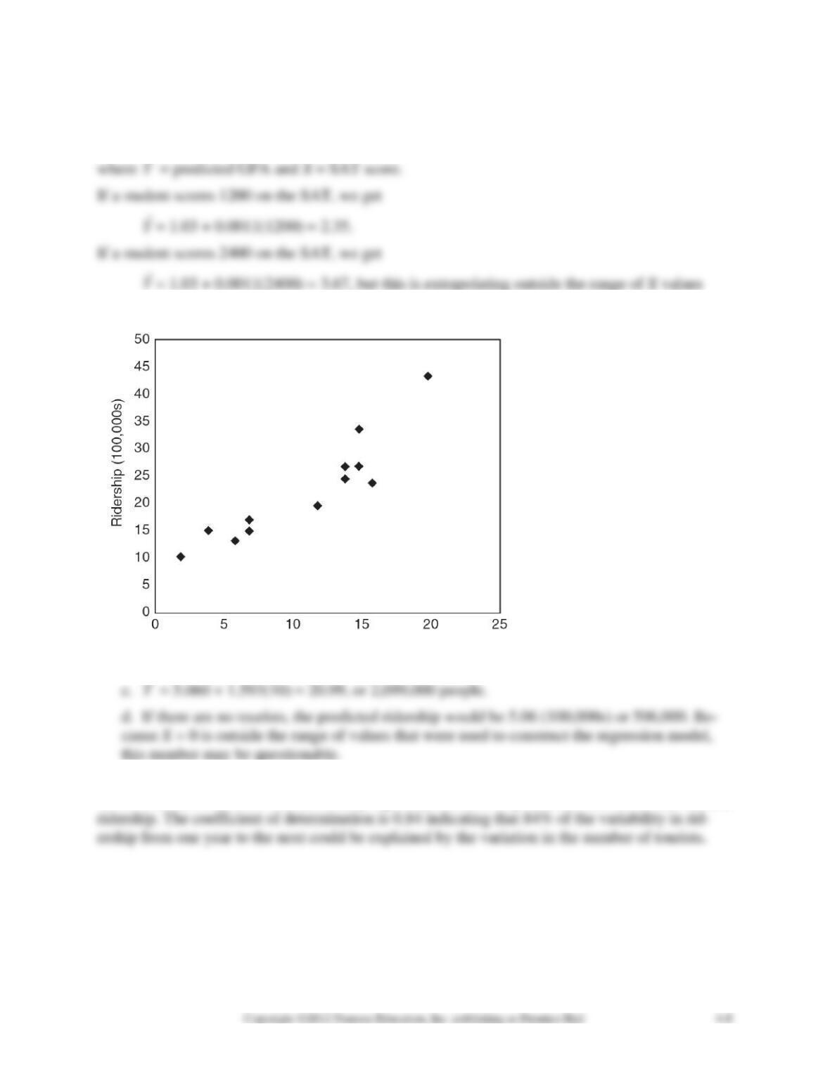
4-19. a. A linear model is reasonable from the graph below.
b.
ˆ
Y
= 5.060 + 1.593X
4-20. The F-value for the F-test is 52.6 and the significance level is extremely small (0.00002)
which indicates that there is a statistically significant relationship between number of tourists and
4-21. a.
ˆ
Y
= 24,328 + 3026.67X1 + 6684X2
where
ˆ
Y
predicted starting salary; X1 = GPA; X2 = 1 if business major, 0 otherwise.
b.
ˆ
Y
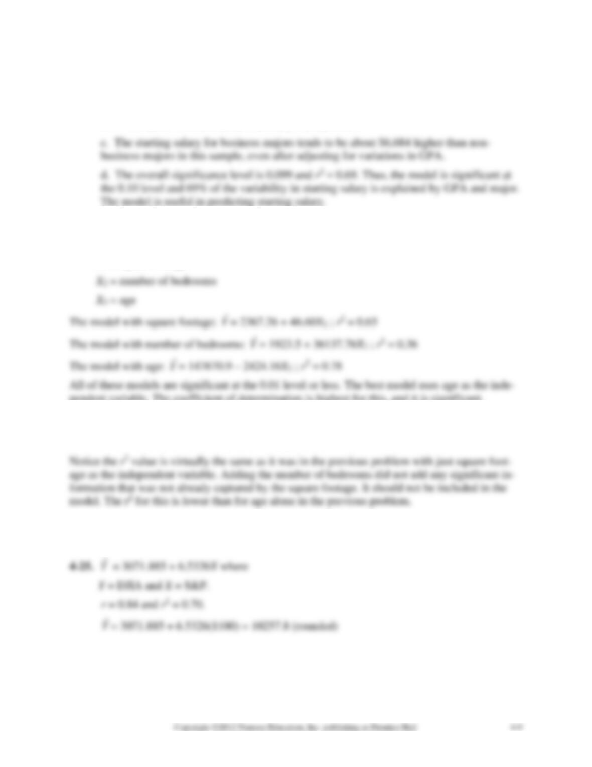
= 24,328 + 3026.67(3.0) + 6684(1) = $40,092.01.
4-22. a. Let
ˆ
Y
ˆ
Y
ˆ
Y
ˆ
Y
= predicted selling price
X1 = square footage
pendent variable. The coefficient of determination is highest for this, and it is significant.
4-23.
ˆ
Y
= 5701.45 + 48.51X1 – 2540.39X2 and r2 = 0.65.
ˆ
Y
= 5701.45 + 48.51(2000) – 2540.39(3) = 95,100.28.
4-24.
ˆ
Y
= 82185.5 + 25.94X1 – 2151.7X2 – 1711.5X3 and r2 = 0.89.
ˆ
Y
ˆ
Y
ˆ
Y
= 82185.5 + 25.94(2000) – 2151.7(3) – 1711.5(10) = $110,495.4.
ˆ
Y
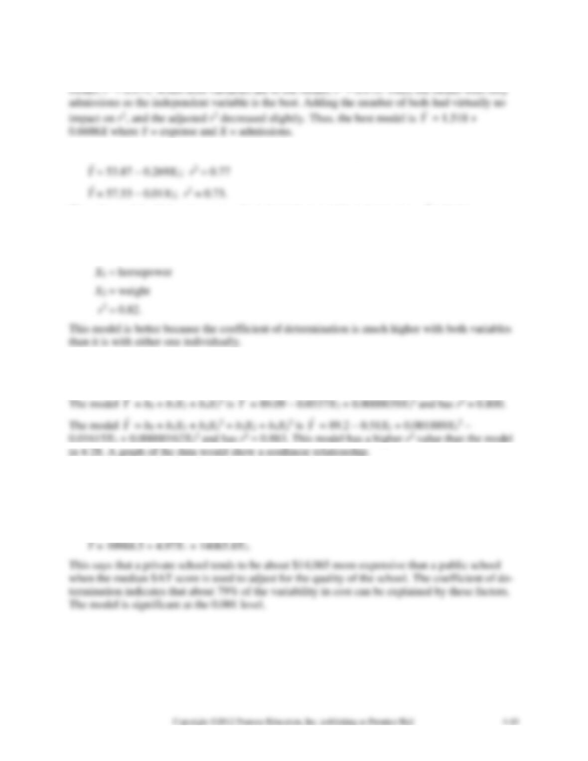
4-26. With one independent variable, beds, in the model, r2 = 0.88. With just admissions in the
4-27. Using Excel with Y = MPG; X1 = horsepower; X2 = weight the models are:
ˆ
Y
ˆ
Y
Thus, the model with horsepower as the independent variable is better since r2 is higher.
4-28.
ˆ
Y
= 57,69 – 0.17X1 – 0.005X2 where
Y = MPG
4-29. Let Y = MPG; X1 = horsepower; X2 = weight
The model
ˆ
Y
= b0 + b1X1 + b2X12 is
ˆ
Y
ˆ
Y
ˆ
Y
ˆ
Y
ˆ
Y
= 69.93 –0.620X1 + 0.001747X12 and has r2 = 0.798.
4-30. If SAT median score alone is used to predict the cost, we get
ˆ
Y
= –11364.7 + 21.6X1 with r2 = 0.22 and a significance level of 0.049.
If both SAT and a dummy variable (X2 = 1 for private, 0 otherwise) are used to predict the cost,
we get r2 = 0.79. The model is
ˆ
Y
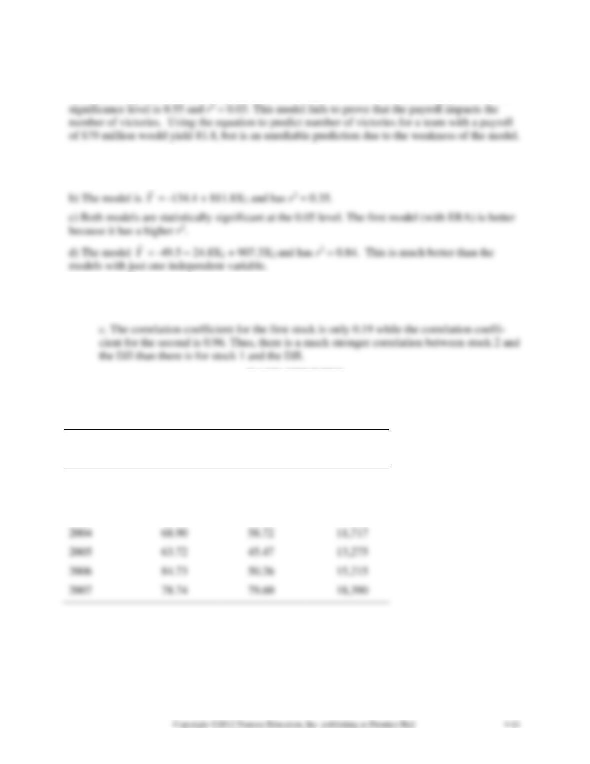
4-31. Y = 78.4 + 0.0436X
There is no significant relationship between the number of victories (Y) and the payroll (X). The
4-32. Let Y = number of wins; X1 = ERA; X2 = batting average
a) The model is
ˆ
Y
= 182.2 – 22.5X1 and has r2 = 0.41.
4-33. a.
ˆ42.43 0.0004YX=+
b.
ˆ31.54 0.0058YX= − +
CASE STUDIES
SOLUTION TO NORTH–SOUTH AIRLINE CASE
Northern Airline Data
Airframe Cost
Engine Cost
Average Age
Year
per Aircraft
per Aircraft
(Hours)
2001
51.80
43.49
6,512
2002
54.92
38.58
8,404
2003
69.70
51.48
11,077
2004
68.90
58.72
11,717
2005
63.72
45.47
13,275
2006
84.73
50.26
15,215
2007
78.74
79.60
18,390
Southeast Airline Data
Airframe Cost
Engine Cost
Average Age
Year
Per Aircraft
per Aircraft
(Hours)
2001
13.29
18.86
5,107
2002
25.15
31.55
8,145
2003
32.18
40.43
7,360
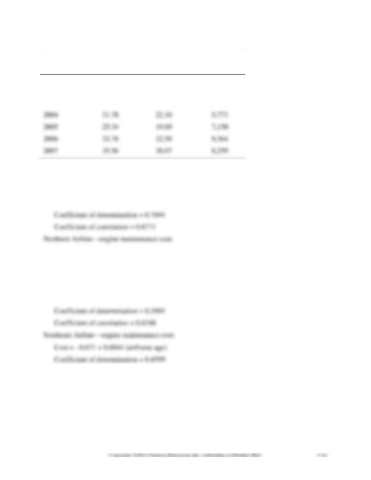
2004
31.78
22.10
5,773
2005
25.34
19.69
7,150
2007
35.56
38.07
8,259
Utilizing QM for Windows, we can develop the following regression equations for the variables
of interest.
Northern Airline—airframe maintenance cost:
Cost = 36.10 + 0.0025 (airframe age)
Cost = 20.57 + 0.0026 (airframe age)
Coefficient of determination = 0.6124
Coefficient of correlation = 0.7825
Southeast Airline—airframe maintenance cost:
Cost = 4.60 + 0.0032 (airframe age)
Coefficient of correlation = 0.6782
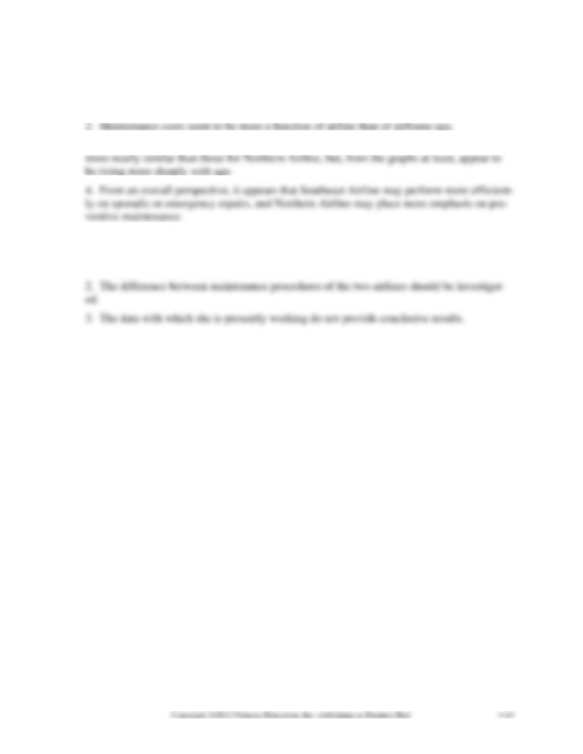
The graphs below portray both the actual data and the regression lines for airframe and en-
gine maintenance costs for both airlines. Note that the two graphs have been drawn to the same
scale to facilitate comparisons between the two airlines.
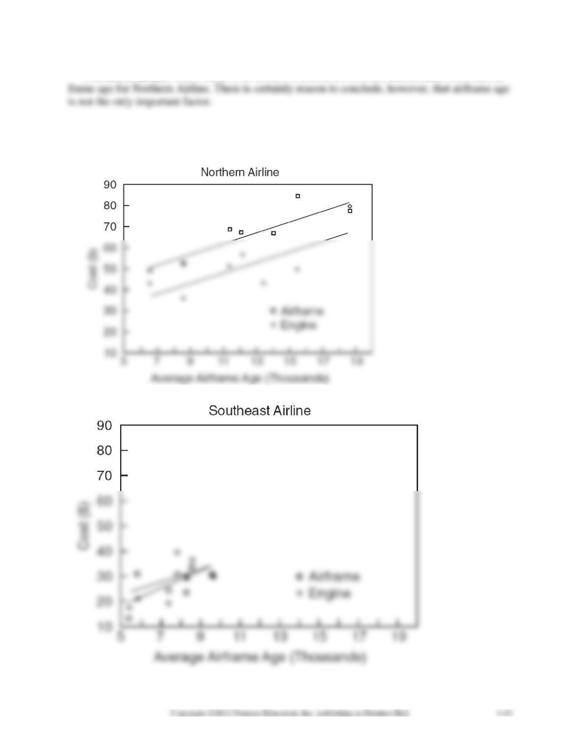
Northern Airline: There seem to be modest correlations between maintenance costs and air-
Southeast Airline: The relationships between maintenance costs and airframe age for South-
east Airline are much less well defined. It is even more obvious that airframe age is not the only
important factor—perhaps not even the most important factor.
Overall, it would seem that:
1. Northern Airline has the smallest variance in maintenance costs, indicating that the day-
to-day management of maintenance is working pretty well.
3. The airframe and engine maintenance costs for Southeast Airline are not only lower but
Ms. Jones’s report should conclude that:
1. There is evidence to suggest that maintenance costs could be made to be a function of air-
frame age by implementing more effective management practices.