
EXERCISE 4-5 4-41
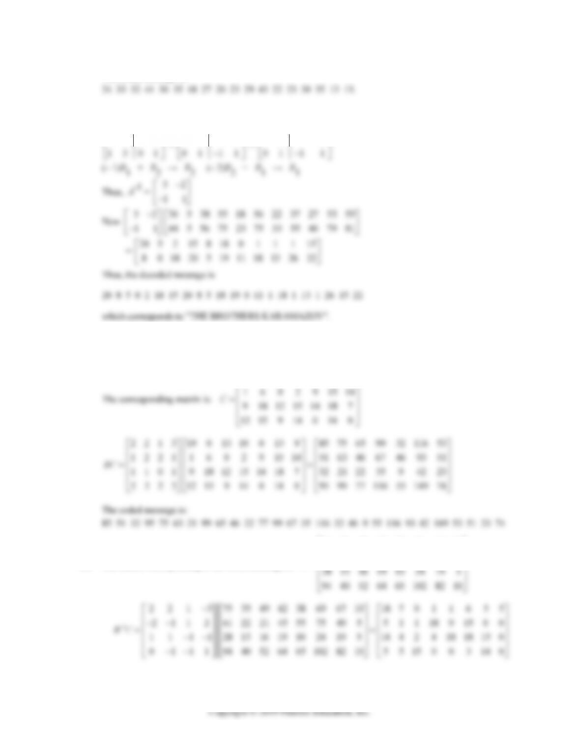
The coded message is:
80. First we must find the inverse of A = 12
13
1210
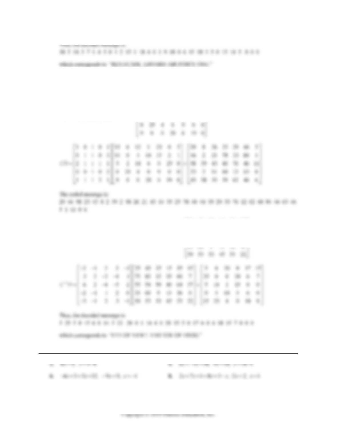
82. “SAIL FROM LISBON IN MORNING” corresponds to the sequence
19 1 9 12 0 6 18 15 13 0 12 9 19 2 15 14 0 9 14 0 13 15 18 14 9 14 7
19 0 13 19 0 13 9
84. The matrix corresponding to the coded message is:
75 35 49 42 38 69 67 10
61 22 21 45 55 75 49 5
C

4-42 CHAPTER 4: SYSTEMS OF LINEAR EQUATIONS; MATRICES
86. “ONE IF BY LAND AND TWO IF BY SEA” corresponds to the sequence:
15 14 5 0 9 6 0 2 25 0 12 1 14 4 0 1 14 4 0 20 23 15 0 9 6 0 2 25 0 19 5 1
The corresponding matrix is:
15 6 12 1 23 0 5
14 0 1 14 15 2 1
5 2 14 4 0 25 0
D
88. The matrix corresponding to the coded message is:
25 43 25 15 35 15
75 83 13 35 60 7
55 54 59 40 64 37
D
EXERCISE 4-6

EXERCISE 4-6 4-43
10. 1
2
21 5
34 7
x
x
x
x
12.
210
231
403
1
2
3
x
x
x
=
6
4
7
x
14. 2x1 + x2 = 8
x
x
x
16. 3x1 + 2x3 = 9
x
x
x
x
18. 1
x
x
= 21
3
= (2)(3) (1)(2)
= 8
1
Thus, 8
x
x
x
2
Thus, 7
x
22. 13
14
1
2
x
x
= 9
6
x
x

4-44 CHAPTER 4: SYSTEMS OF LINEAR EQUATIONS; MATRICES
x
x
24. 11
32
1
2
x
x
= 10
20
x
x
1110
3201
~ 1110
0531
~ 1
3
01
~
1
3
01
0.6 0.2
2
x
x
0.6 0.2
20
2
Therefore, x1 = 8, x2 = 2.
26. 21
13
1
2
x
x
+ 3
5
= 10
16
or 21
13
1
2
x
x
= 7
11
x
x
2110 1301 1 30 1
~ 12
13 0 1
x
x
28. 34
68
1
2
x
x
+ 1
0
= 2
1
or 34
68
1
2
x
x
= 1
1
EXERCISE 4-6 4-45
30. 32
21
1
2
x
x
– 4
1
= 4
3
or 32
21
1
2
x
x
= 8
4
x
x
12
2101 01
2101
~
012 3
x
x
32. The matrix equation for the given system is:
x
x
k
From Exercise 4-5, Problem 42, 21
-1
= 31
x
x
(A) 1
2
x
x
= 31
52
13
= 7
16
1
2
and 16
x
x
x
x
x
34. The matrix equation for the given system is:
x
x
k
From Exercise 4-5, Problem 44, 21
-1
= 11
x
x
4-46 CHAPTER 4: SYSTEMS OF LINEAR EQUATIONS; MATRICES
(A) 1
x
x
= 11
1
= 1
1
Thus, 1
x
x
x
x
x
36. The matrix equation for the given system is:
230
1
x
x
x
1
k
From Exercise 4-5, Problem 46,
230
12 3
-1
=
7159
5106
3
x
x
x
3
1
x
x
x
7159
5106
0
2
39
26
3
x
x
x
121
1
3
1
x
x
x
7159
3
6
38. The matrix equation for the given system is:
10 1
1
x
x
x
1
k
10 1
-1
211

EXERCISE 4-6 4-47
Thus,
1
x
x
x
211
1
k
3
x
x
x
31 1
0
4
1
x
x
x
211
4
12
x
x
x
40. Cannot divide by a matrix, 1
XBA
.
42. Must multiply on the left. 1
XAB
.
44. Matrix multiplication is not commutative. 1
XABA
.
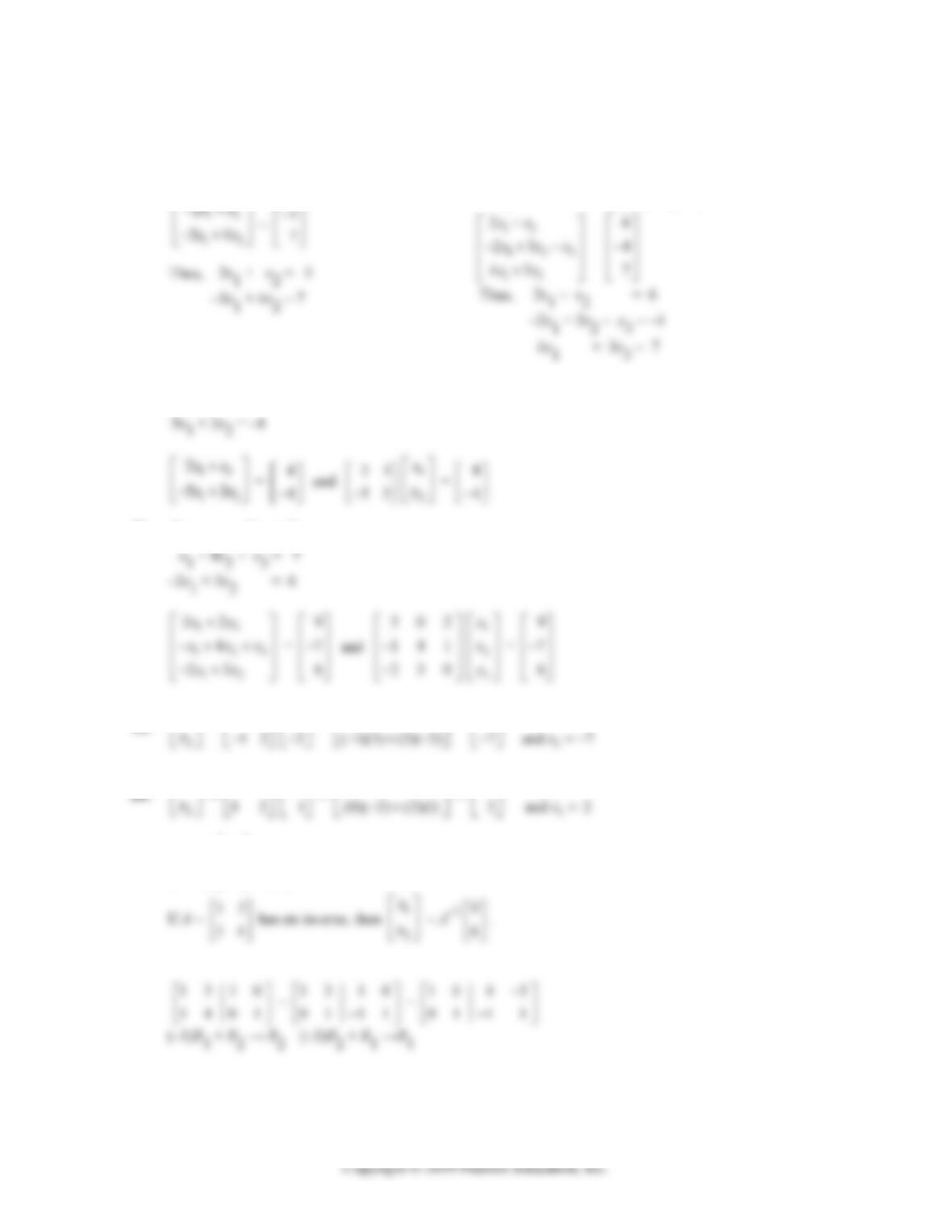
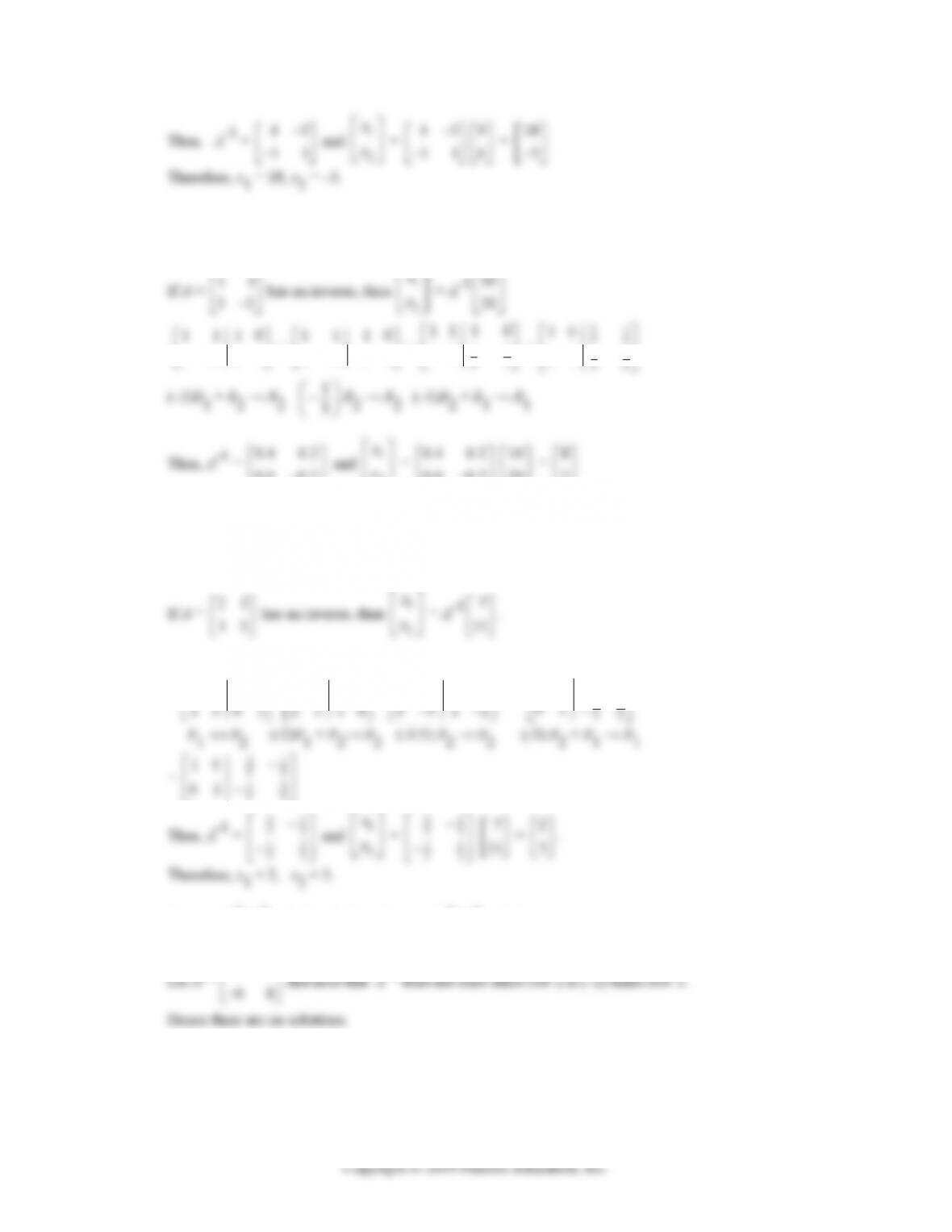
46. –2x1 + 4x2 = 5 (1)
48. x1 – 3x2 – 2x3 = –1
–2x1 + 7x2 + 3x3 = 3
The system is not “square”– 2 equations with 3 unknowns. The matrix of coefficients is 2 × 3; it does not
have an inverse.

4-48 CHAPTER 4: SYSTEMS OF LINEAR EQUATIONS; MATRICES
50. x1 – 2x2 + 3x3 = 1 (1)
52. AX + BX = C
(A + B)X = C
54. AX – X = C
56. AX + C = BX + D
AX – BX = D – C
58. 11 1
22 2
51 32 20 23 20
is the same as
2 2 1 3 31 3 5 31
xx x
xx x
60. The matrix equation for the given system is:
727
1
x
x
x
59
x
x
x
62. The matrix equation for the given system is:
21 65
1
x
x
x
x
54

EXERCISE 4-6 4-49
Thus
1
x
x
x
x
21 65
-1 54
5.9
1
5.9
x
64. (A) Let x1 = Number of local vehicles
x2 = Number of non-local vehicles
The mathematical model is:
57.5
2
x
x
2
k
Compute the inverse of the coefficient matrix A.
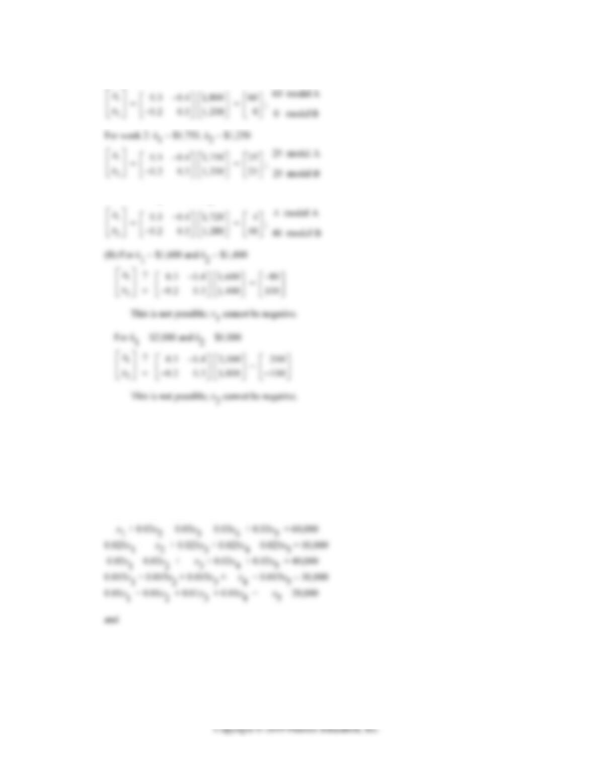
Day 1: k1 = 1,200, k2 = $7,125
x
x
Day 2: k1 = 1,550, k2 = $9,825
x
x
Day 3: k1 = 1,740, k2 = $11,100
x
x
Day 4: k1 = 1,400, k2 = $8,650
x
x
4-50 CHAPTER 4: SYSTEMS OF LINEAR EQUATIONS; MATRICES
(B) k2 = $5,000
x
x
This is not possible; x2 cannot be negative.
x
x
This is not possible; x1 cannot be negative.
Letting x2 = t, we have x1 = 1200 – t. Substituting for x1 and x2 in (2) we obtain
66. (A) Let x1 = number of model A guitars produced
x2 = number of model B guitars produced
Then, the mathematical model is:
30x1 + 40x2 = k1 (Labor allocation)
20x1 + 30x2 = k2 (Materials allocation)
x
x
First we compute the inverse of 30 40
20 30
41
41
01 0.20.3
01 0.2 0.3
-1
x
x
k
EXERCISE 4-6 4-51
Now, for week 1: k1 = $1,800, k2 = $1,200
For week 3: k1 = $1,720, k2 = $1,280
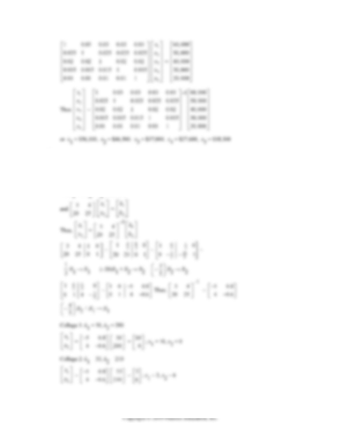
68. Let x1 = President’s bonus
x2 = Executive Vice President’s bonus
x3 = Associate Vice President’s bonus
x4 = Assistant Vice President’s bonus
x5 = Sales Manager’s bonus
Then, the mathematical model is:
4-52 CHAPTER 4: SYSTEMS OF LINEAR EQUATIONS; MATRICES
70. Let x1 = Number of lecturers hired
x2 = Number of instructors hired
The mathematical model is:
3x1 + 4x2 = k1 (sections)
20x1 + 25x2 = k2 (salaries)

EXERCISE 4-7 4-53
EXERCISE 4-7
10. 20¢ from A and 10¢ from E
12. I – M = 10
01
– 0.4 0.2
0.2 0.1
= 0.6 0.2
0.2 0.9
0.4 1.2
x
x
14. X = 1
x
x
= (I – M)-1D2 = 1.8 0.4
0.4 1.2
12
9
= 25.2
15.6
.
16. 30¢ for A, 20¢ for B, 20¢ for E.
18. I – M =
100
010
–
0.3 0.2 0.2
0.1 0.1 0.1
=
0.7 0.2 0.2
0.1 0.9 0.1
20. X = (I – M)-1D2
1
x
x
x
1.6 0.4 0.4
20
42

4-54 CHAPTER 4: SYSTEMS OF LINEAR EQUATIONS; MATRICES
24. I – M = 10
01
– 0.4 0.1
0.2 0.3
= 0.6 0.1
0.2 0.7
26. I – M =
100
010
001
–
0.3 0.2 0.3
0.1 0.1 0.1
0.1 0.2 0.1
=
0.7 0.2 0.3
0.1 0.9 0.1
0.1 0.2 0.9
1290010
1290010

EXERCISE 4-7 4-55
79 20 90
10 0
00 10
11 11 11
(–2)R2+R1→R1 11
500 R3→R3
(79/11)R3+R1→R1
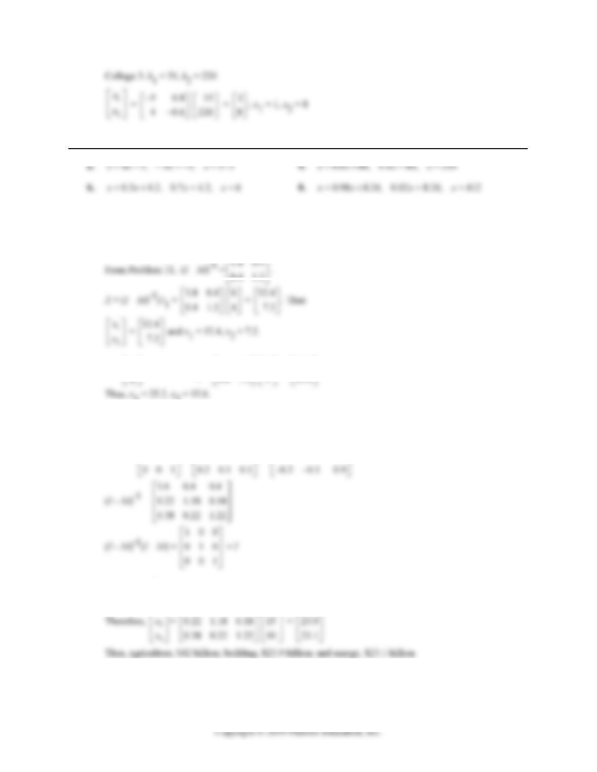
28. (A) The technology matrix M = 0.25 0.25
0.4 0.2
and the final demand matrix
The solution is X = (I – M)-1D, provided I – M has an inverse. Now,
4-56 CHAPTER 4: SYSTEMS OF LINEAR EQUATIONS; MATRICES
0.8 1.5
2
x
x
0.8 1.5
50
115
0.4 0.8
90
82
30. The technology matrix T = 0.2 0.4
0.25 0.25
and the final demand D is given by D = 50
50
(see Problem 28).
0.25 0.25
50
2
x
x
01
0.25 0.25
0.25 0.75
0.25 0.75 0 1
0.25 0.75 0 1
0.8
0 0.625 0.3125 1
010.51.6
010.51.6
0.625
0.5 1.6
x
x
0.5 1.6
50
105
32. Let x1 = total output of automobiles, and
x2 = total output of construction
2
0.70
x
x
EXERCISE 4-7 4-57
2
x
x
0.1 0.1
2
x
x
2
0.70
x
x
or
0.2 0.1
x
x
x
or x1 = 2x2 which is a dependent case.
36. The technology matrix M = 0.1 0.4
0.1 0.4
and the final demand matrix
0.1 0.4
20
2
x
x
01
0.1 0.4
0.1 0.6
0.1 0.6 0 1
0.1 0.6 0 1
38. The technology matrix M = 0.40 0.20
0.35 0.05
and the final demand matrix
x
x
01
0.35 0.05
0.35 0.95

4-58 CHAPTER 4: SYSTEMS OF LINEAR EQUATIONS; MATRICES
0.35 0.95 0 1
15
0.35 0.95 0 1
1
0.6 R1 → R1 (0.35)R1 + R2 → R2
0.7 1.2
2
x
x
0.7 1.2
250
328
40. The technology matrix M =
0.3 0.3 0.1
0.1 0.1 0.1
0.2 0.2 0.1
and the final demand matrix D =
25
15
20
.
The input-output matrix equation is X = MX + D.
0.1 0.9 0.1 0 1 0
~
77
7
0.1 0.9 0.1 0 1 0
77
7
4
61
010
~
77
7
27
1
01 0
~
EXERCISE 4-7 4-59
131
522
10 0
3
11
522
10 0
1001.580.580.24
5R3→R3 1
5
R3 + R1 → R1
X =
2
x
x
x
=
0.22 1.22 0.16
15
=
27
.
42. The technology matrix is M =
0.14 0.07 0.21 0.24
0.15 0.13 0.31 0.19
.
The input-output matrix equation is X = MX + D
A
E
M
0.15 0.13 0.31 0.81
X =(I – M)-1D
18
50
Year 2: D =
31
19
and (I – M)-1D =
82
57
4-60 CHAPTER 4: SYSTEMS OF LINEAR EQUATIONS; MATRICES
37
89
CHAPTER 4 REVIEW
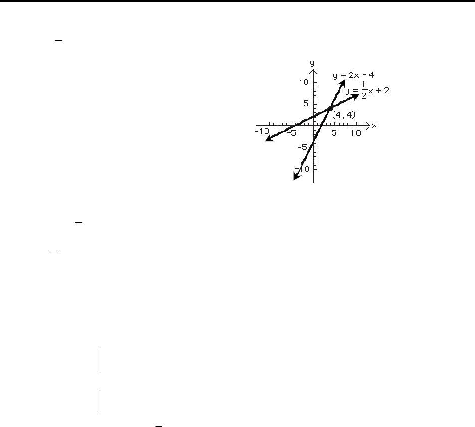
1. y = 2x – 4 (1)
y = 1
2. Substitute equation (1) into (2):
2x – 4 = 1
2x + 2
3. (A) 012
103
is not in reduced form; the left-most 1 in the second row is not to the right
of the left-most 1 in the first row. [condition 4] R1 ↔ R2