
College Mathematics: Learning Worksheets Chapter 4
Name ________________________________ Date ______________ Class ____________
Goal: To solve systems of linear equations in two variables
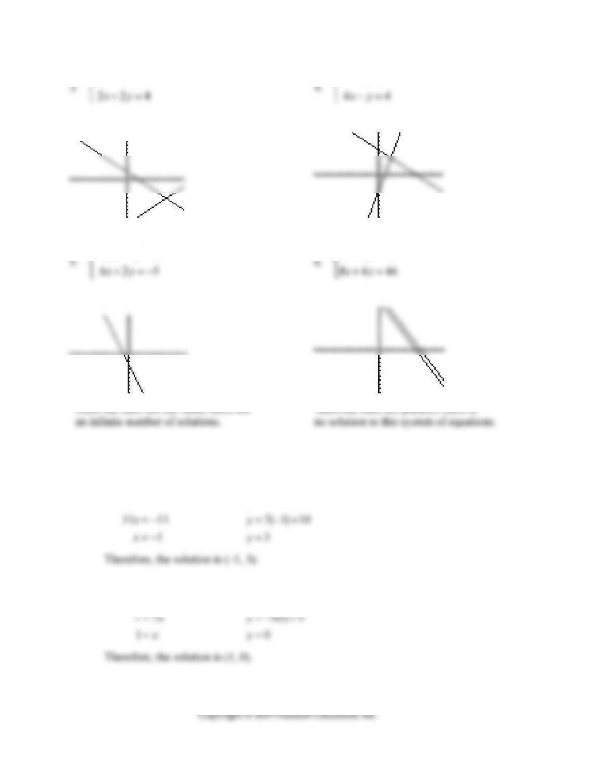
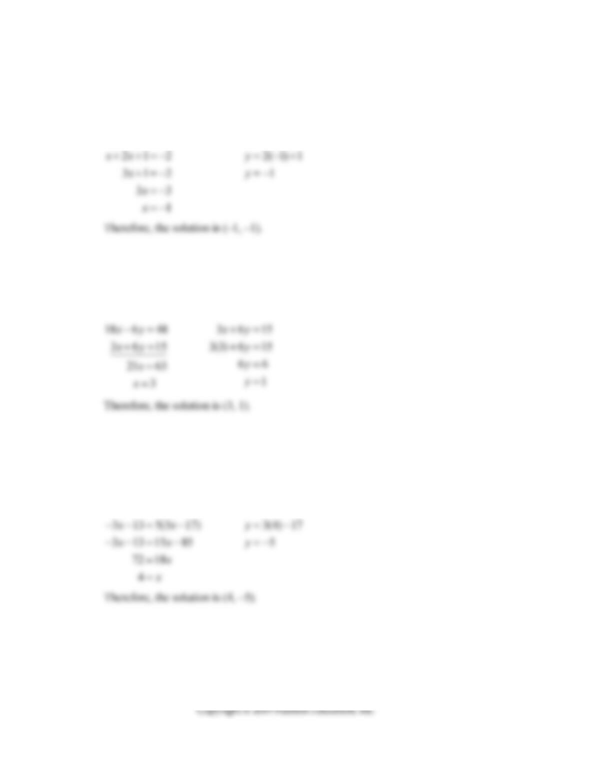
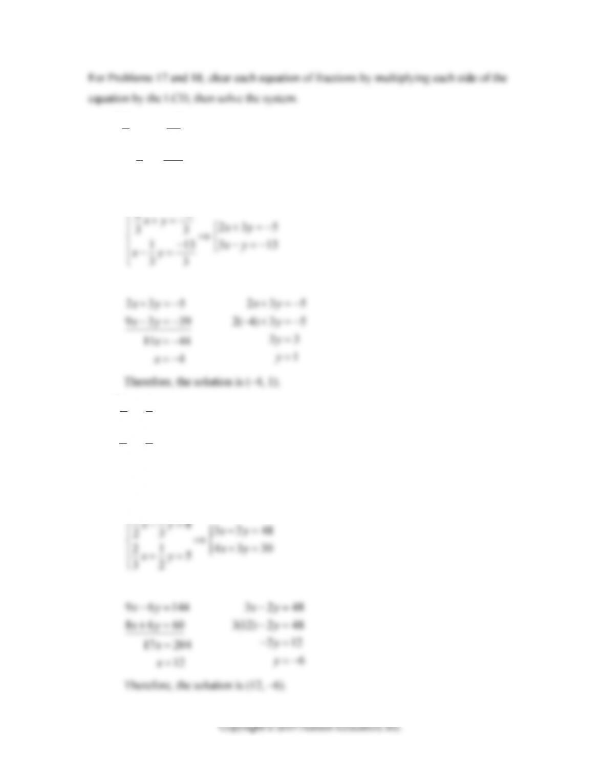
In Problems 1–6, solve the systems of equations by graphing:
1. 710
yx
=+
⎧
⎨=− −
yx
Section 4-1 Review: Systems of Linear Equations
in Two Variables
Solving Systems of Equations:
Method 1: Substitution
2. Substitute the equation found in step 1 into the other equation.
4. Substitute the answer from step 3 into the original equation used in step 1 to find
the value of the other variable.
Method 2: Addition
1. Get both equations in standard form ( ax by c)
3. Add the two equations together to eliminate one variable.
5. Substitute the answer from step 4 into either original equation to find the value of
the other variable.
College Mathematics: Learning Worksheets Chapter 4
104
xy
3318
xy
Point of intersection is (7, –5). Point of intersection is (2, 4).
xy
−−=
⎧
63 39
xy
+=
⎧
Since the lines are the same, there are Since the lines are parallel, there is
For Problems 7–12, solve the Problems in 1–6 by algebraic methods.
7. 710 41
x
x
+=−−
710
yx
=+
8. 5522
xx
55
yx
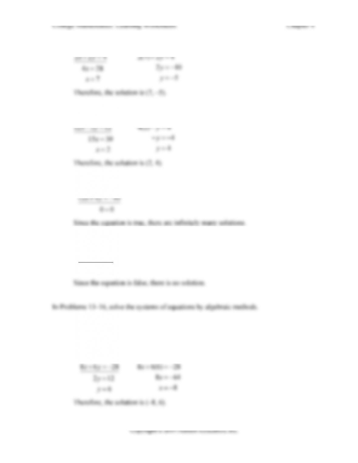
105
9. 22 24
xy
22 4
xy
10. 3318
xy
44
xy
11. 12 4 10
xy
−−=
12. 42 26
42 23
03
xy
xy
−− =−
+=
=−
13. 42 20
86 28
xy
xy
+=−
⎧
⎨+=−
⎩
84 40
xy
−− =
86 28
xy
+=−
College Mathematics: Learning Worksheets Chapter 4
106
14. 21
2
y
x
xy
2
xy
21
yx
15. 93 24
3615
xy
xy
−=
⎧
⎨+=
⎩
16. 317
3135
yx
x
y
3135
xy
317
yx
College Mathematics: Learning Worksheets Chapter 4
107
17.
25
33
113
33
xy
xy
Multiply both equations by 3:
25
23 5
33
xy xy
18.
118
23
215
32
xy
xy
Multiply both equations by 6:
11832 48
xy xy
108
19. Suppose the supply and demand for posters of the 2017 Super Bowl Champions for a
particular week are
p
p
q Supply Equation
=+
where p is the price in dollars and q is the quantity in thousands.
a) Find the supply and demand (to the nearest unit) if the posters are priced at $6.
Supply: Demand:
0.8 2.6
pq
=+
1.2 9
pq
=− +
If the price is $6, the supply will be 4250 posters and the demand will be 2500
posters.
b) Find the supply and demand (to the nearest unit) if the posters are priced at $8.
Supply: Demand:
80.8 2.6
5.4 0.8
6.75
q
q
q
=+
=
=
81.29
11.2
0.833
q
q
q
=− +
−=−
=
If the price is $8, the supply will be 6750 posters and the demand will be 833 posters.
c) Find the equilibrium price and quantity.
0.8 2.6 1.2 9
qq
+=− +
0.8 2.6
pq
=+
The equilibrium price is $5.16 when the supply and demand both are 3200 posters.
109
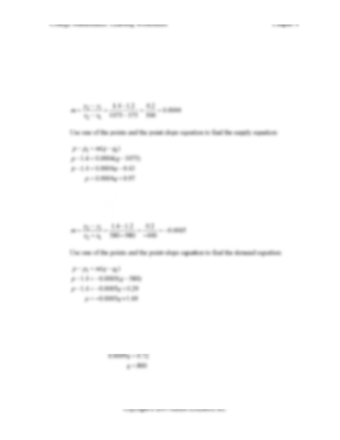
20. At $1.40 per pound, the daily supply of tobacco is 1075 pounds and the daily demand is
580 pounds. When the price falls to $1.20 per pound, the daily supply decreases to 575
pounds and the daily demand increases to 980 pounds. Assume that the supply and demand
equations are linear.
a) Find the supply equation.
Use the two supply points, (1075, 1.4) and (575, 1.2), to find the slope of the line:
1.4 0.0004( 1075)
1.4 0.0004 0.43
0.0004 0.97
pq
pq
pq
b) Find the demand equation.
Use the two demand points, (580, 1.4) and (980, 1.2), to find the slope of the line:
1.4 0.0005( 580)
1.4 0.0005 0.29
0.0005 1.69
pq
pq
pq
c) Find the equilibrium price and quantity.
0.0004 0.97 0.0005 1.69
qq
110
College Mathematics: Learning Worksheets Chapter 4
Name ________________________________ Date ______________ Class ____________
Goal: To solve systems of linear equations using augmented matrices
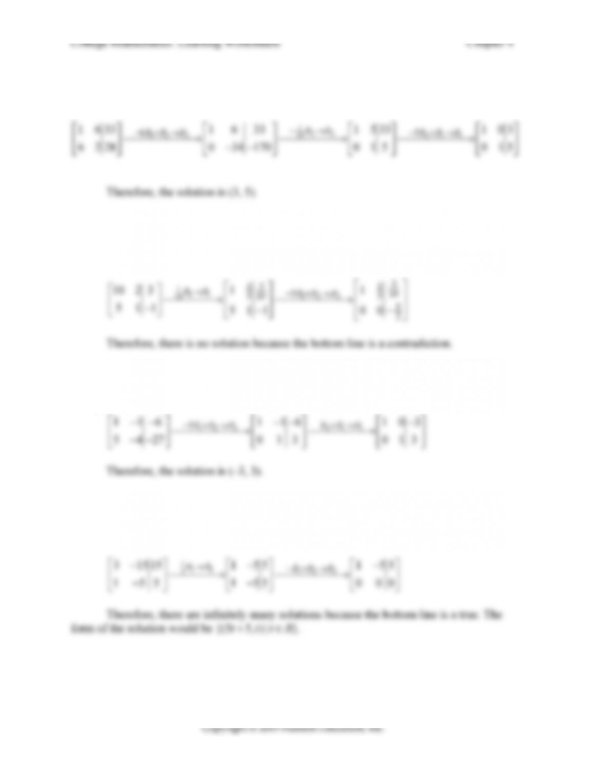
Solve the following systems of linear equations by augmented matrix methods.
1. 22 2
62 2
xy
xy
−=−
⎧
⎨−=−
⎩
2. 210
23 1
xy
xy
122
1 2 10 1 2 10 1 2 10 1 0 4
RR
Section 4-2 Systems of Linear Equations and
Augmented Matrices
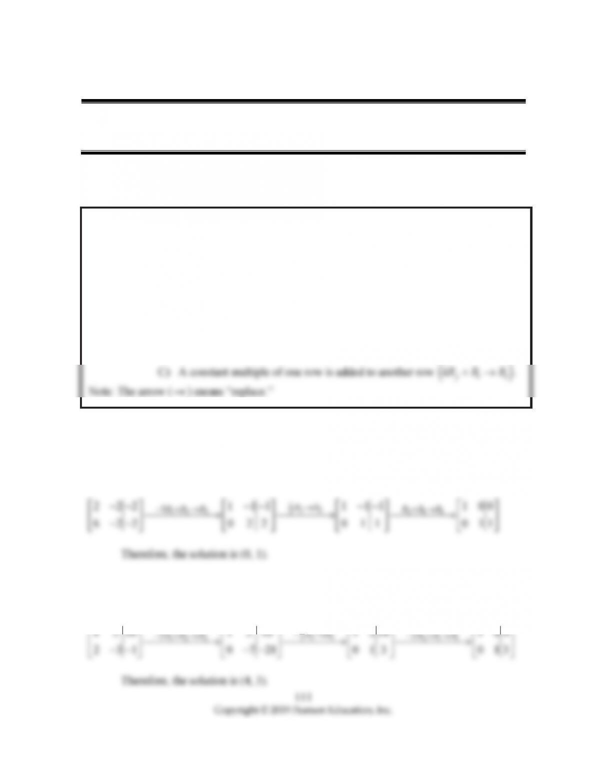
Operations That Produce Row-Equivalent Matrices
An augmented matrix is transformed into a row-equivalent matrix by performing any
of the following row operations:
A) Two rows are interchanged
ij
R
R.
B) A row is multiplied by a nonzero constant
ii
kR R.
112
3. 633
62 28
xy
xy
+=
⎧
⎨+=
⎩
4. 10 2 3
51
xy
xy
111
10 1 2 2
3
3
11
510
55
10
11
10 2 3
RR RR R
5. 6
54 27
xy
xy
−=−
⎧
⎨−=−
⎩
5
116 116 103
RR R R R R−+→ +→
⎡⎤ ⎡⎤ ⎡⎤
−− −− −
6. 315 15
55
xy
xy
111
3122
31515 155 155
RR RR R
College Mathematics: Learning Worksheets Chapter 4
113
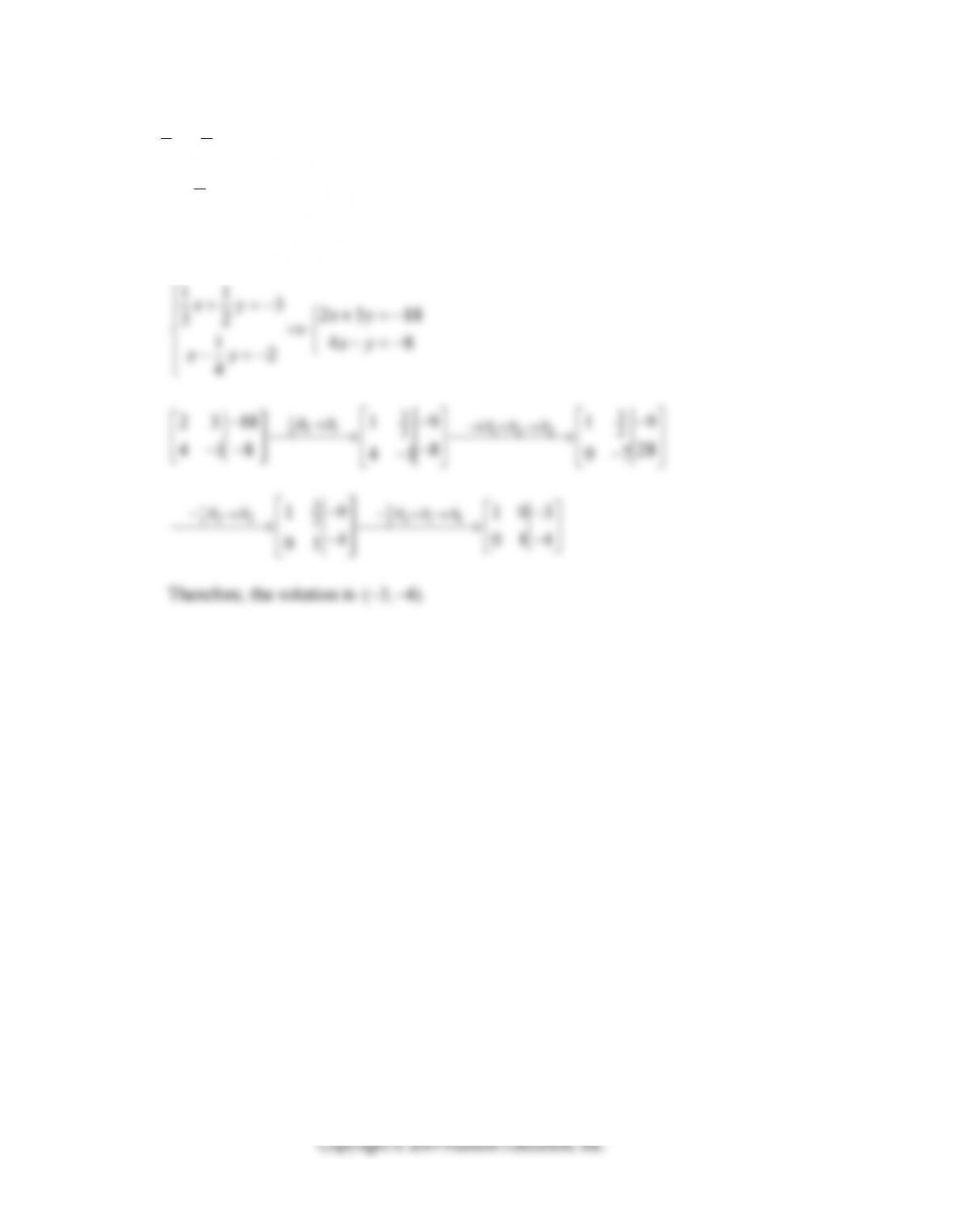
7.
55
22
4615
yx
xy
Multiply the first equation by 2 and put the first equation in standard form:
55 52 5
22 4615
4615
xy
yx
xy
xy
2
2
8. 512
10 2 12
xy
xy
−+=
⎧
⎨−=−
⎩
9. 32
42 3
xy
xy
12
10 10
College Mathematics: Learning Worksheets Chapter 4
114
10. 28 9
46
xy
xy
3
2
146 14 00
6
Therefore, there is no solution because the bottom line is a contradiction.
11. 32 4
64 8
xy
xy
−=
⎧
⎨−+ =−
⎩
12. 34
2
xy
xy
111
3122
14
14 33
33
1
1
314
RR RR R
College Mathematics: Learning Worksheets Chapter 4
115
13. 23 4
5616
xy
xy
14. 45 2
12 15 6
xy
xy
42
College Mathematics: Learning Worksheets Chapter 4
116
15.
11 3
32
12
4
xy
xy
First multiply equation 1 by 6 and equation 2 by 4 to remove the fractions:
11 323 18
32
xy xy

College Mathematics: Learning Worksheets Chapter 4
117
Name ________________________________ Date ______________ Class ____________
Goal: To solve systems of equations using the Gauss-Jordan Elimination method
Section 4-3 Gauss-Jordan Elimination
A matrix is said to be in reduced row form if
1. Each row consisting entirely of zeros is below any row having at
least one nonzero element.
3. All other elements in the column containing the leftmost 1 of a
given row are zeros.
4. The leftmost 1 in any row is to the right of the leftmost 1 in the row above.
Gauss-Jordan Elimination
Step 1. Choose the leftmost nonzero column and use appropriate row
operations to get a 1 at the top (element 11
a).
Step 3. Move to column 2 and use appropriate row operations to get a 1 in the
position of the element of the principal diagonal (element 22
a).
Step 5. Continue in this manner until all the elements of the principal diagonal
are one (with zeros elsewhere in the column).
Note: If at any point in this process we obtain a row with all zeros to the left of
College Mathematics: Learning Worksheets Chapter 4
118
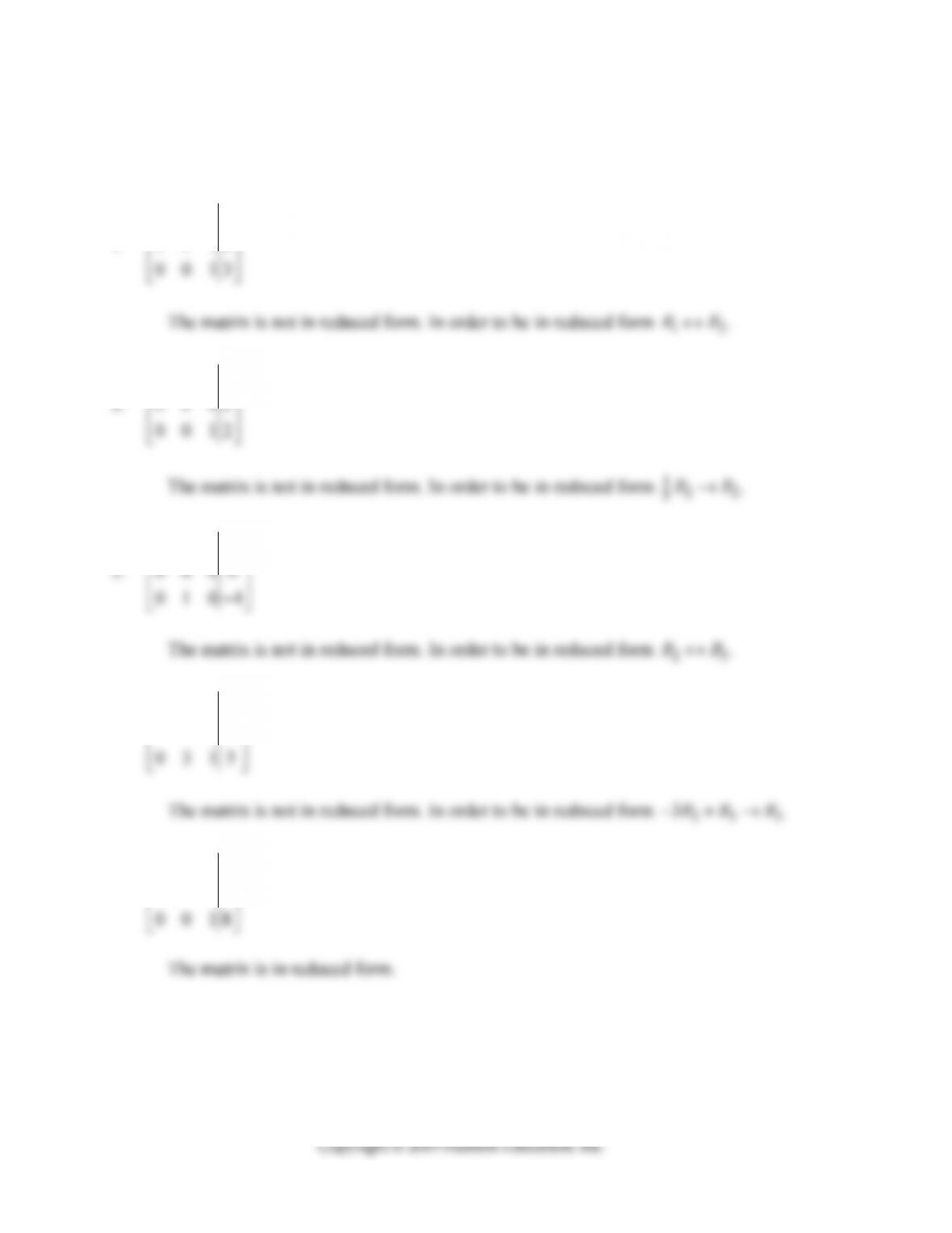
In Problems 1–5, determine if the matrices are in reduced form. If the matrix is not in
reduced form explain (symbolically) the row operation(s) necessary to transform the matrix
into reduced form.
1.
0102
1008
⎡⎤
⎢⎥
1003
⎡⎤
⎢⎥
5.
1005
4.
1002
01012
⎡⎤
⎢⎥
⎢⎥
5.
1003
0109
College Mathematics: Learning Worksheets Chapter 4
119
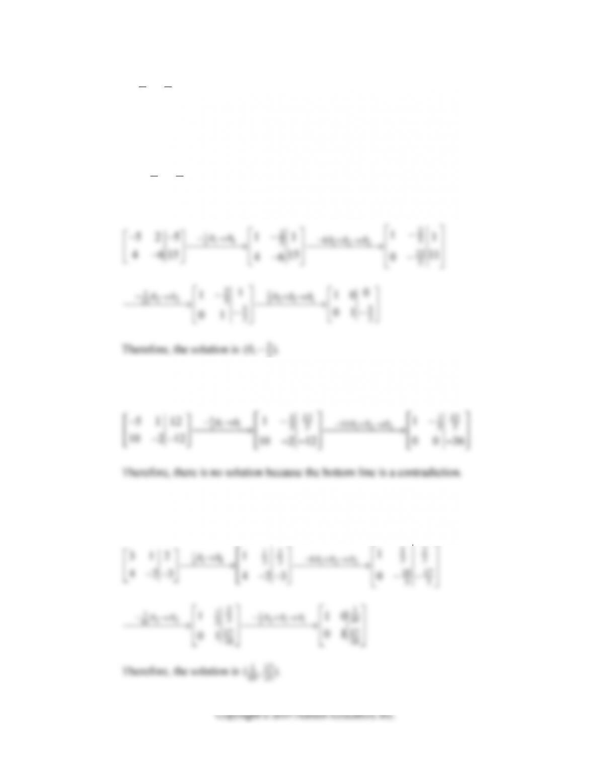
In Problems 6–13, solve the problems using Gauss-Jordan elimination.
6. 12
12
24
32 6
xx
xx
111 12 2
1
132
1
214 1 2 2
RR RR R
7. 12
12
57
36 0
xx
xx
157 1 57 1 57
8. 12
12
35 3
610 10
xx
xx
35
College Mathematics: Learning Worksheets Chapter 4
120
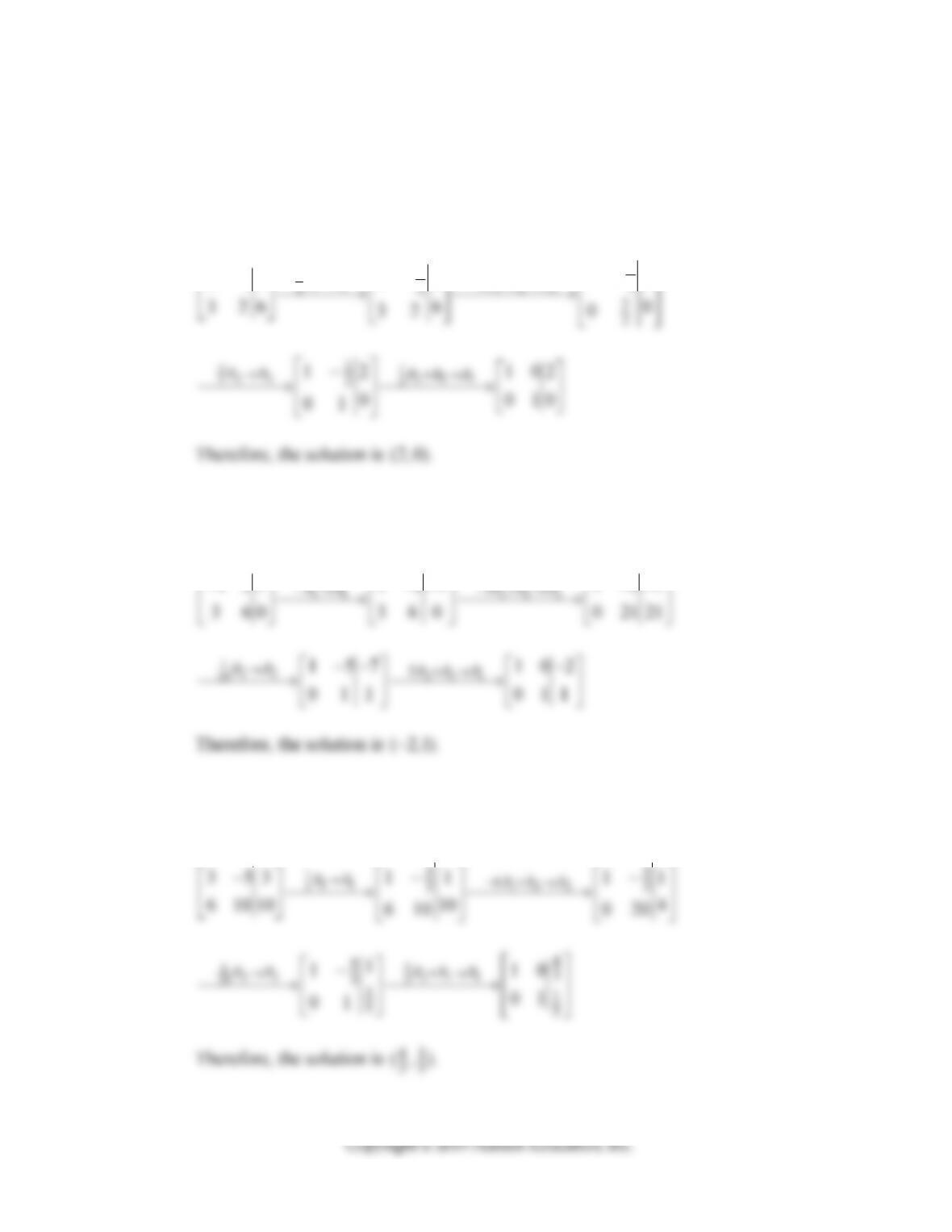
9. 12
12
311
25 4
xx
xx
111
111
111 233
1
1
3111
RR RR R
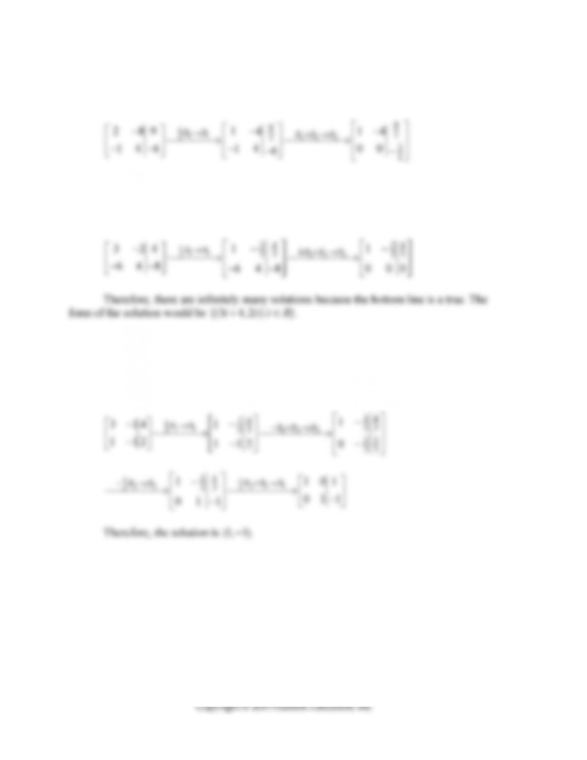
10.
2x1−x2=−4
2x1+4x2=6
3x1−x2=−1
1
122
11
22
2
11
214 2 2
1
12101
College Mathematics: Learning Worksheets Chapter 4
121
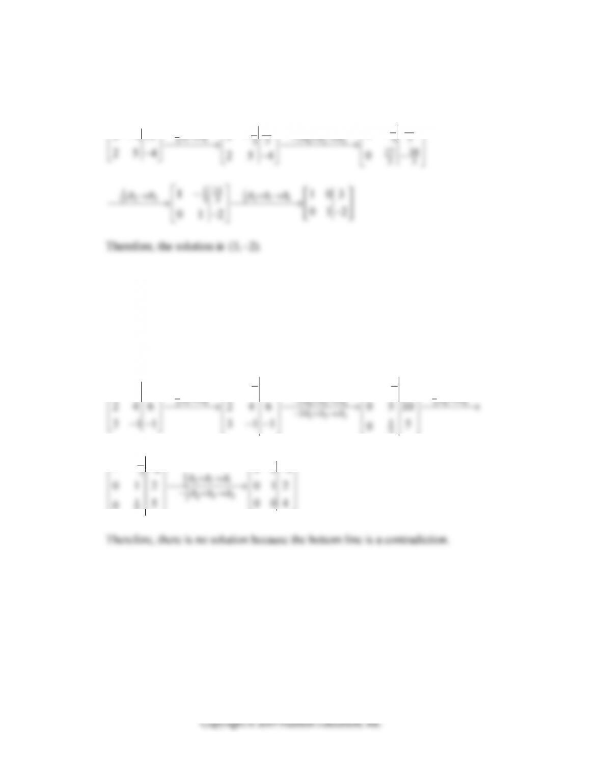
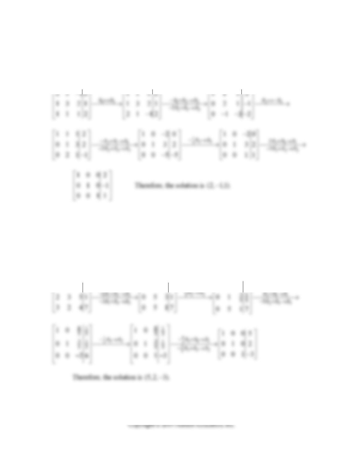
11.
2x1+x2−x3=2
x1+3x2+2x3=1
x1+x2+x3=2
21 12 11 12 1 1 12
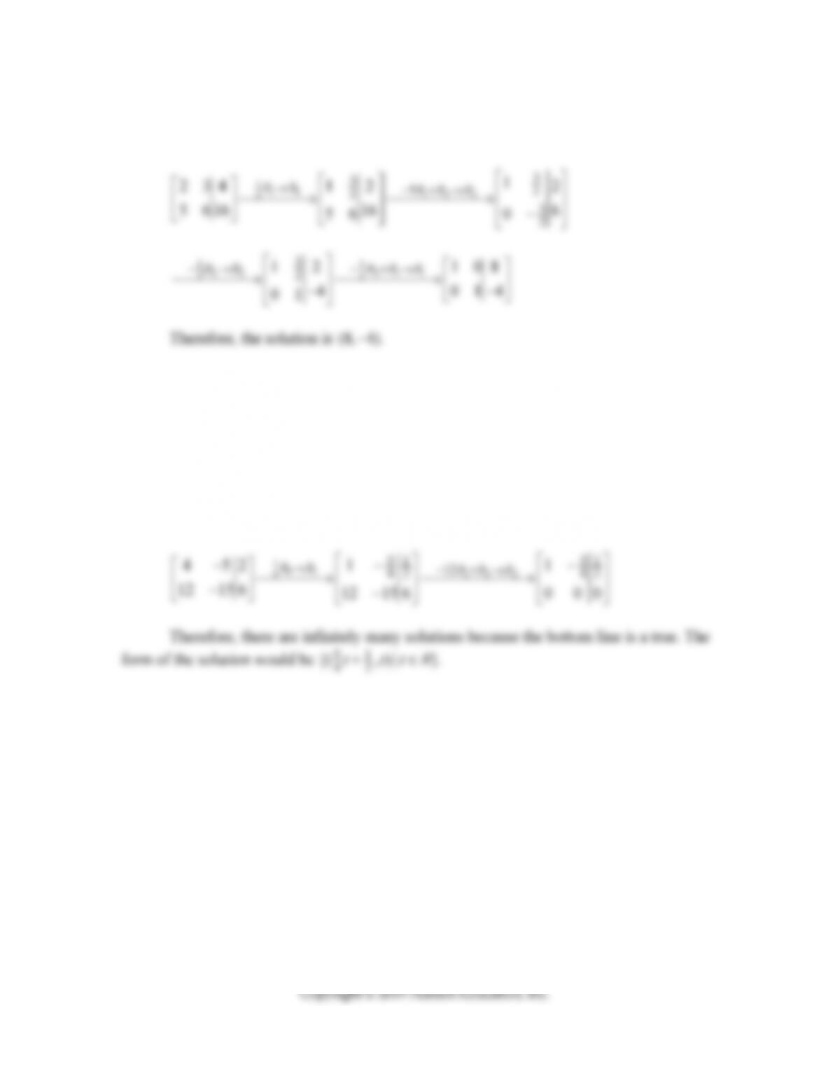
12.
x1−x2+x3=0
2x1+3x2+5x3=1
3x1+2x2+4x3=7
111
0
1110 1110
College Mathematics: Learning Worksheets Chapter 4
122
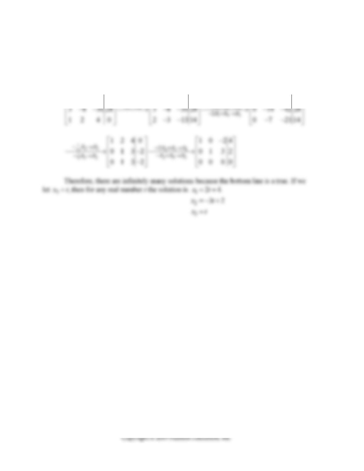
13.
12 3
12 3
123
2 3 13 14
3 8 30 28
240
xx x
xx x
xx x
2 3 13 14 1 2 4 0 1 2 4 0
x
2
3
32
x
t
xt
=− +
=