Management Chapter 3 We then establish Little's law to set up other

13

CHAPTER 3: PROCESS FLOW MEASURES

3.1 Objective

The objective of this chapter is to identify key operational measures that may be used to study process

flows. They are linked together using Little’s law. We then present a series of examples that show how

3.2 Additional Suggested Readings

We assign a short case as supplemental reading for the analysis of process flows. The case is used to do a

thorough analysis of flows and identify key drivers of cost and revenue in a process. This understanding

is then used to identify actions that improve performance.

3.3 Solutions to the Chapter Questions

Discussion Question 3.1

The opposite of looking at average is looking at a specific flow unit’s flow time, and the inventory status

Discussion Question 3.2

In practice, one often tracks inventory status periodically (each day, week, or month). Flow rate is

14 Chapter 3

Discussion Question 3.3

First, draw a process flow chart.

Second, calculate all operational flows: throughput, inventory, and flow time for each activity.

Third, calculate the financial flow associated with each activity. If the activity incurs a cost (or earns a

Discussion Question 3.4

For the department of tax regulations we have

Average inventory I = 588 projects,

Discussion Question 3.5

If GM and Toyota have same turns, and we know that

Discussion Question 3.6

Yes, low inventories means few flow units are held in the buffer. In contrast, fast inventory turns means

short flow times; i.e., flow units do not spend a long time in the process. As such, one can have high

turns with high or low inventories (it all depends on what the throughput is).

Discussion Question 3.7

A short cost-to-cash cycle means that it does not take long to convert an input into a sold output. Clearly,

Exercise 3.1 (Bank)

For the bank we have

Chapter 3 15

90%

Buffer 1

Registration

Buffer 2

Doctor

Potential admits

10%

Exercise 3.2 (Fast-Food)

For the fast food outlet we have

Exercise 3.3 (Checking Accounts)

For a checking account we have

Exercise 3.4 (ER)

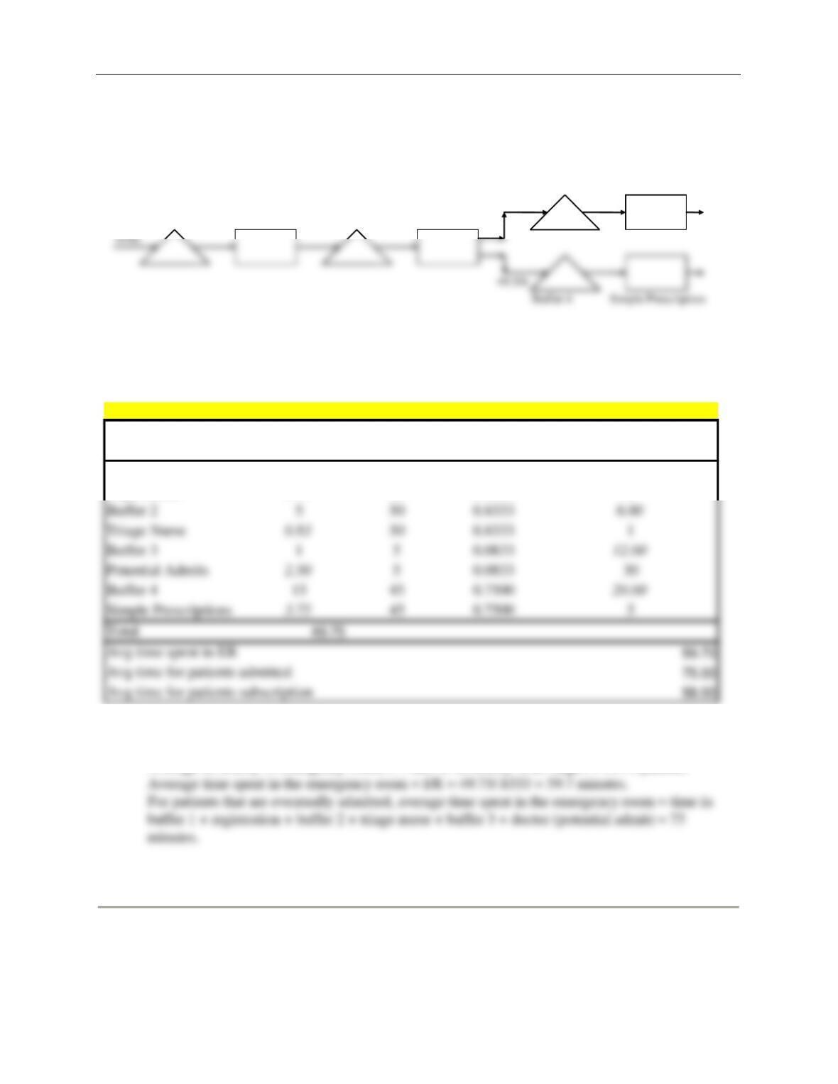
First draw the flowchart with all the data given:

We assume a stable system. This implies that average inflow equals average outflow at every stage. In

this case you are given inventory numbers I and flow rate R = 55 patients/hr. There are two flow units:

(1) Those that are potential admits: flow rate = 55*10% = 5.5/hr.

16 Chapter 3

(1) Buffer 1: R = 55/hr (both flow units go through there), I = 7, so that waiting time in buffer 1 =

T = I/R = 7/55 hr = 0.127 hours = 7.6 minutes.

OK, now we have everything to find the total average flow times: find the critical path for each flow unit.

In this case, each flow unit only has one path, so that is the critical path. We find its flow time by adding

the activity times on the path:

The answer to the other questions is found as follows:

1. On average, how long does a patient spend in the emergency room?

2. On average, how many patients are being examined by a doctor?

This question asks for the average inventory at the doctor’s activity. Again, first calculate inventory of

each type of flow unit:

3. On average, how many patients are in the ER?

Chapter 3 17

Buffer 1

Registration

Buffer 2

Triage Nurse

Buffer 3

Potential admits

5.5/hr

Exercise 3.5 (ER, triage)

The process flow map with the triage system is as follows:

The inventory, and time spent in various locations are as follows. In each case the calculated quantity is

italicized.

Throughput through ER, R = 55 patients / hour = .8333/min.

Average inventory in emergency room, I = sum of inventory in all stages = 49.75 patients

Exercise 3.6 (ER, triage with misclassification)

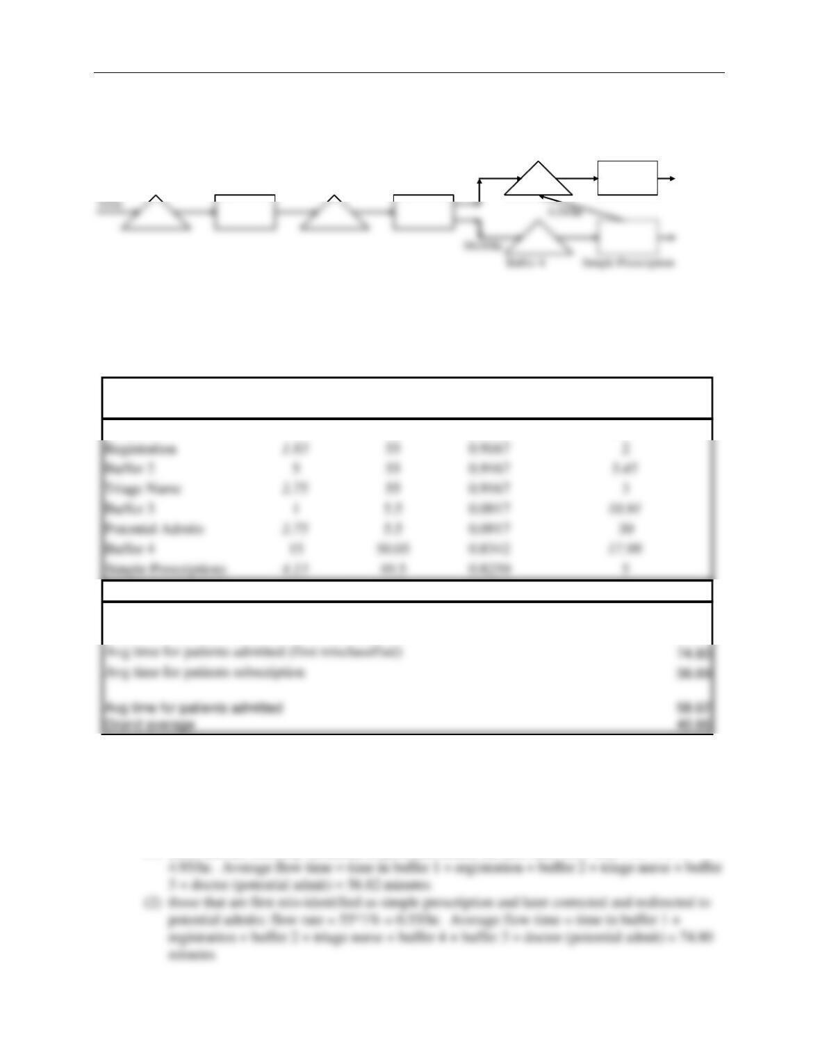
In this case the process flow map is altered somewhat since there are some patients sent from simple

prescriptions to buffer 3.

Exercise 3.5

Location

Inventory

Throughput

(per hr)

Throughput

(per min)

Flow Time (min)

Buffer 1

20 50 0.8333 24.00

Registration

1.67 50 0.8333 2

18 Chapter 3

Buffer 1

Registration

Buffer 2

Triage Nurse

Buffer 3

Potential admits

4.95/hr

(We will assume that the doctor “instantaneously” recognizes misclassification so that a misclassified

patient does not spend 5 minutes with the doctor. However, if you assume such person also spends 5

minutes, the entire methodology below follows, only increase the relevant flow time by 5 minutes.)

The inventories, throughputs and flow times are as follows:

Throughput through ER, R = 55 patients / hour

Average inventory in emergency room, I = sum of inventories in all stages = 37.46

Average time spent in the emergency room T = I/R = 37.46/.9167 = 40.86 minutes.

To calculate flow times, we should distinguish three types of flow units:

(1) those that are correctly identified as potential admits the first time: flow rate = 55*9% =

Location

Inventory

Throughput

(per hr)

Throughput

(per min)

Flow Time (min)

Buffer 1

555 0.9167 5.45

Total 37.46

Avg time spent in ER 40.86

Avg time for patients admitted (correctly classified) 56.82

55/hr

50.05/hr

0.55/hr

Chapter 3 19

(3) those that are correctly identified to get a simple prescription the first time: flow rate =

55*90% = 49.5/hr. Average flow time = time in buffer 1 + registration + buffer 2 + triage

nurse + buffer 4 + buffer 3 + doctor (simple prescription) = 38.89 minutes

Exercise 3.7 (Orange Juice Inc)

First let us notice that there are two periods in the day:

1. From 7am-6pm, oranges come in at a rate of 10,000kg/hr and are processed, and thus leave the plant,

at 8000kg/hr. Because inflows exceed outflows, inventory will build up at a rate of

20 Chapter 3

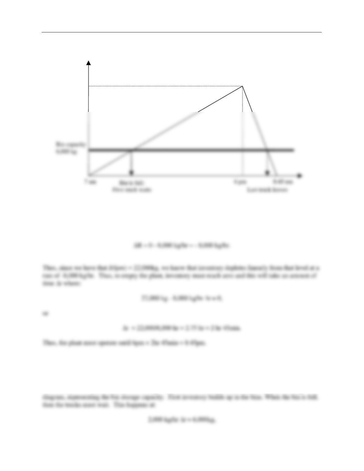
Inventory I (t)

22,000 kg

2. After 6pm, no more oranges come in, yet processing continues at 8000 kg/hr until the plant is empty.

Thus, inflows is less than outflows so that inventory is depleted at a rate of

This can all be graphically summarized in the inventory build up diagram shown above.

3. Truck dynamics: for this the inventory diagram is really useful. Notice that we have taken a total

process view of the plant, including the truck waiting queue. Thus, inventory is total inventory in the bins

+ inventory in the trucks (if any are waiting). So, let’s draw the thick line on the inventory build-up

Chapter 3 21

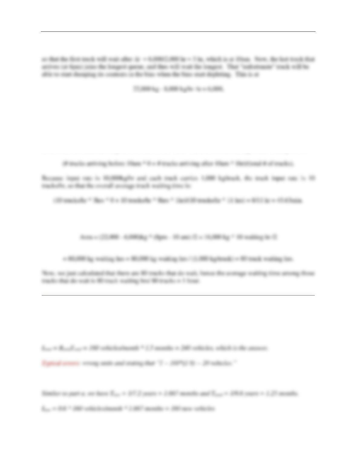
or after t = (22,000-6,000)/8,000 hr = 2 hr, after 6pm. Thus, the last truck departs at 8pm and the

maximum truck waiting time is therefore 2 hours.

Now, among all the trucks that do wait (i.e., those arriving after 10am), the first truck waits practically

zero minutes, and the last truck waits 2 hours, culminating in an average of (0 + 2)hrs/2 = 1 hour.

Notice that the trucks arriving before 10am do not wait. Thus, the overall average truck waiting time is

Average waiting time can also be calculated by noticing that the area of the upper triangle in the build-up

diagram represents the total amount of hours waited by all trucks:

Exercise 3.8 (Jasper Valley Motors)

Part a.

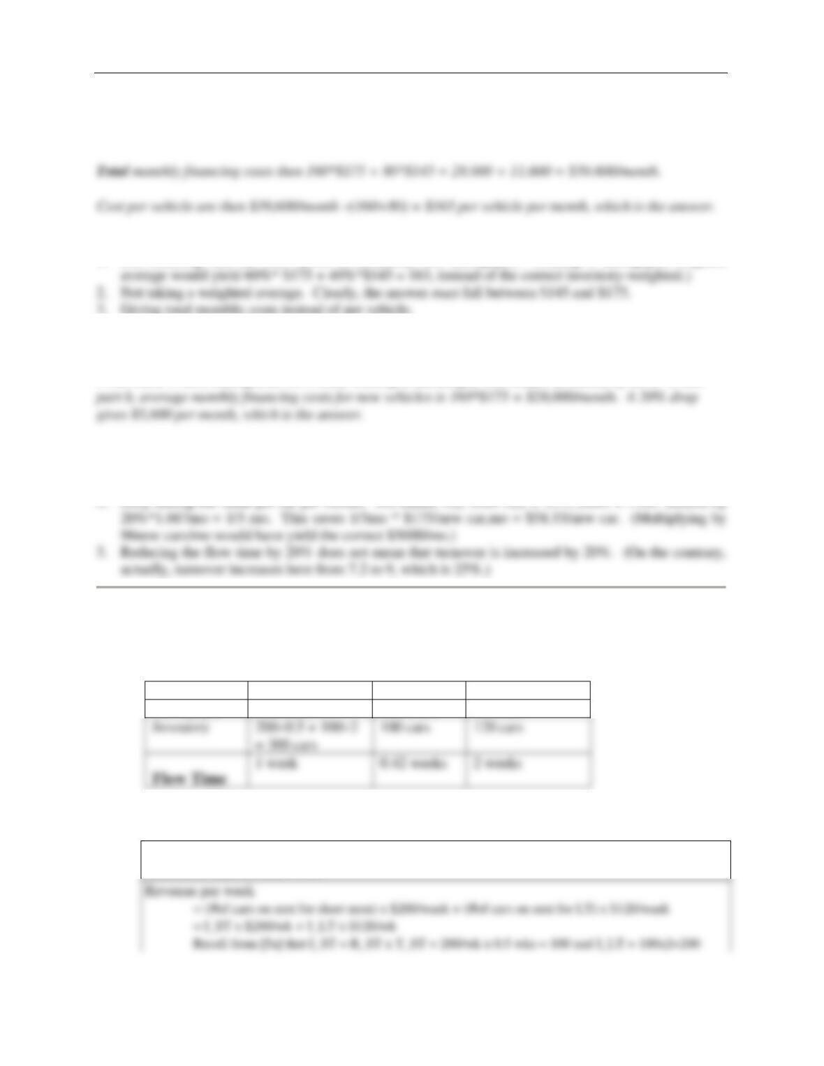
TURNStotal = 1/Ttotal so Ttotal = 1/8 years = 1.5 months

Part b.

22 Chapter 3

Iused = 0.4 * 160 vehicles/month * 1.25 months = 80 new vehicles

Typical errors:

1. Not realizing that the cost driver is inventory, not throughput. (Taking a throughput-weighted

3. Giving total monthly costs instead of per vehicle.

Part c.

From Little’s Law, cutting time 20% while holding R unchanged will reduce inventory by 20%. From

Typical errors:

1. Assuming the service works also on used cars, leading to 20%$39,600/month= $7920/mo.

Exercise 3.9 (Cheapest Car Rentals)

Part a.

Customers

Clean area

Repair area

Throughput

300/week

240/week

60/week

Part b:

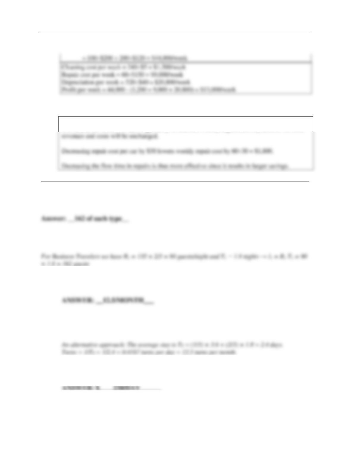
Number of cars owned by Cheapest = 300 + 100 + 120 = 520

Number of cars on rent = 300

Chapter 3 23

Part c:

Decreasing flow time in repairs by 1 week will lower the inventory in repairs from 120 to 60. This

will reduce the number of cars required by 60 and thus weekly depreciation by $2,400. All other

Exercise 3.9 (The Evanstonian)

Part a.

For Leisure Travelers we have:

RL = 135/3 = 45 guests/night and TL = 3.6 nights → IL = RL TL = 45 × 3.6 = 162 guests

× 1.8 = 162 guests

Part b:

The total inventory is then IT = 324. We then have Turns = RT/IT = 135/324 = 0.4167 turns per

day = 12.5 turns per month.

Part c:

24 Chapter 3

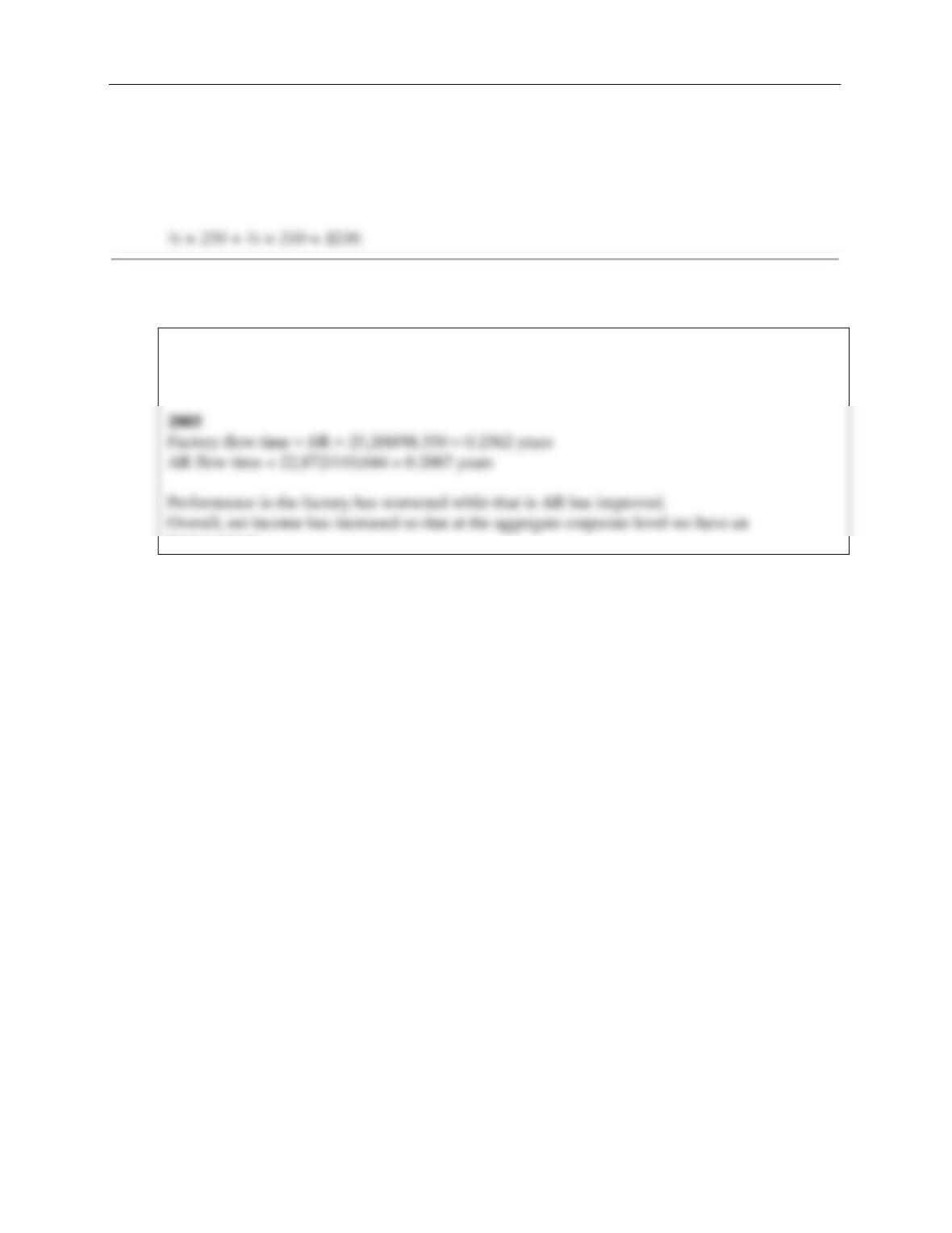
From the analysis above on the average night, 324 rooms are occupied with half of the guests

being leisure travelers. Thus the average rate that The Evanstonian receives per occupied room

is:

Exercise 3.11 (ABC Corporation)

2004

Factory flow time = I/R = 20,880/97,380 = 0.2144 years (must use COGS dollars)

AR flow time = 21,596/99,621 = 0.2168 years (must use sales dollars)

improvement.