Chapter 3
Chapter 3
Probability Distributions
Case Problem: Specialty Toys
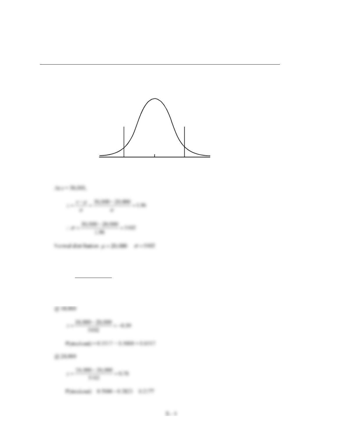
1. Information provided by the forecaster
2. @ 15,000
15,000 20,000 0.98
5102
z−
= = −
P(stockout) = 0.3365 + 0.5000 = 0.8365
20,000
.05
10,000 30,000
.05 .90
Chapter 3
3 –
2
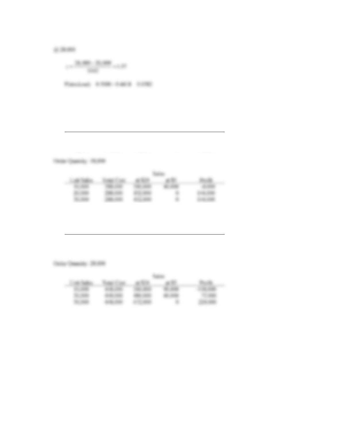
3. Profit projections for the order quantities under the 3 scenarios are computed below:
Order Quantity: 15,000
Sales
Unit Sales
Total Cost
at $24
at $5
Profit
10,000
240,000
240,000
25,000
25,000
20,000
240,000
360,000
0
120,000
30,000
240,000
360,000
0
120,000
Sales
Unit Sales
Total Cost
at $24
at $5
Profit
10,000
288,000
240,000
40,000
20,000
288,000
432,000
0
144,000
30,000
288,000
432,000
0
144,000
Order Quantity: 24,000
Sales
Unit Sales
Total Cost
at $24
at $5
Profit
10,000
384,000
240,000
70,000
-74,000
20,000
384,000
480,000
20,000
116,000
30,000
384,000
576,000
0
192,000
Sales
Unit Sales
Total Cost
at $24
at $5
Profit
10,000
448,000
240,000
90,000
-118,000
20,000
448,000
480,000
40,000
30,000
448,000
672,000
Probability Distributions
3 –
3
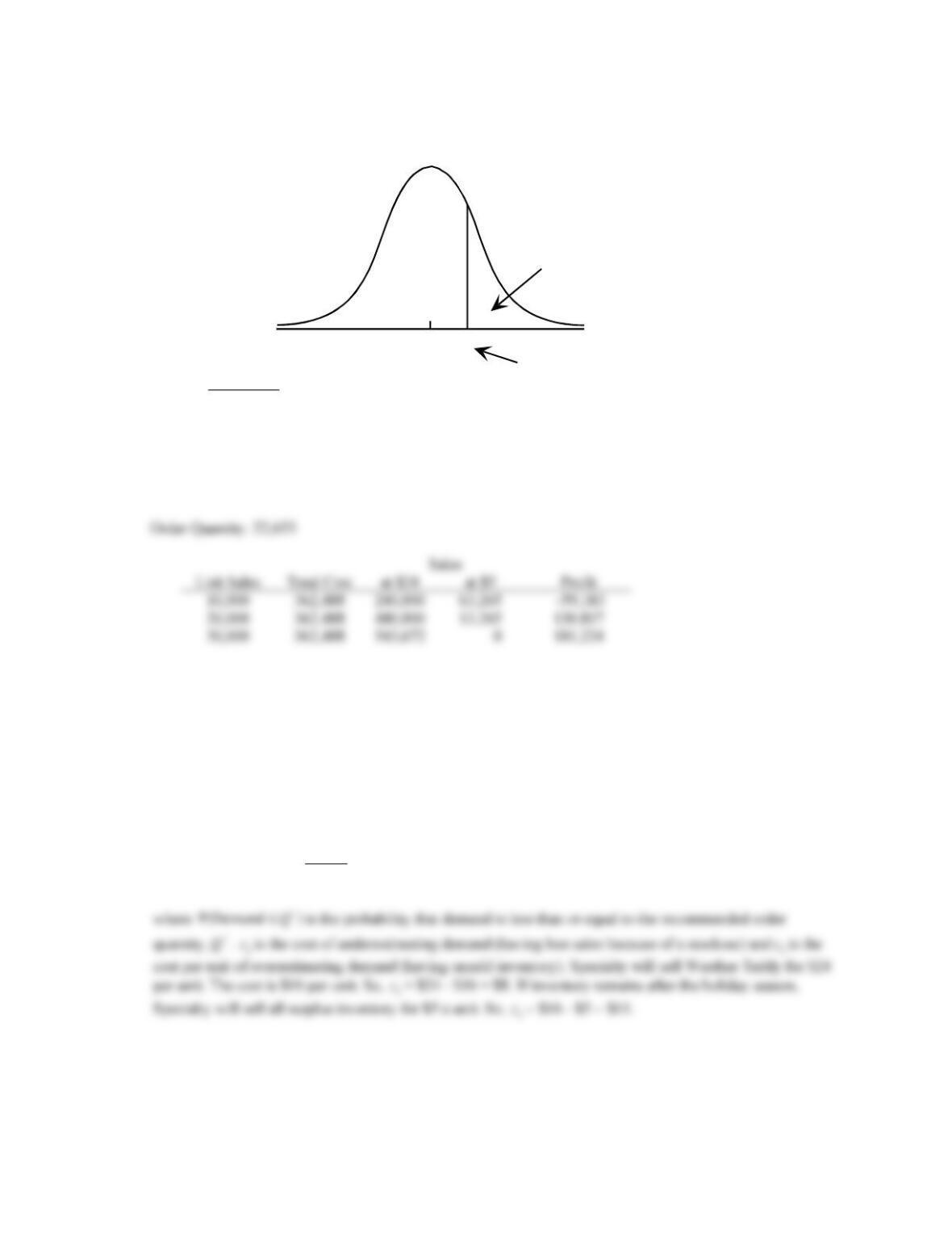
4. We need to find an order quantity that cuts off an area of .70 in the lowest tail of the normal curve for demand.
20,000 0.52
5102
Q
z−
==
Q = 20,000 + 0.52(5102) = 22,653
The projected profits under the 3 scenarios are computed below.
5. A variety of recommendations are possible. The students should justify their recommendation by showing the
projected profit obtained under the 3 scenarios used in parts 3 and 4. An order quantity in the 18,000 to
20,000 range strikes a good compromise between the risk of a loss and generating good profits.
While the students don’t have the benefit of the following, a single-period inventory model (sometimes called
the news vendor model) shows how to find an optimal solution. We outline that solution below.
A single-period inventory model recommends an order quantity that maximizes expected profit based on the
following formula:
*
P(Demand ) u
uo
c
Qcc
=
+
20,000
30%
Qz = 0.52
70%
Chapter 3
3 –
4
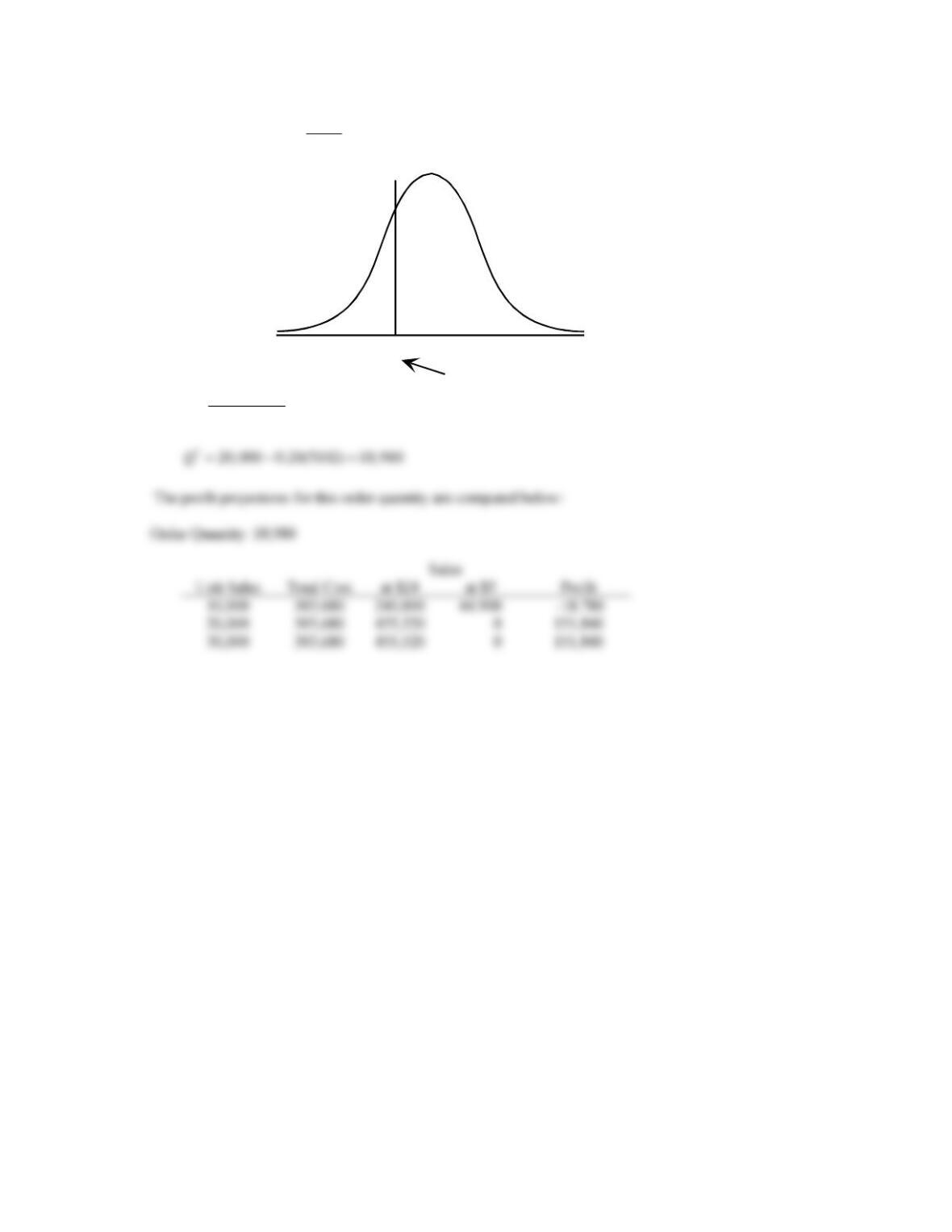
*8
P(Demand ) 0.4211
8 11
Q = =
+
*20,000 0.20
5102
Q
z−
= = −
0.5789
Q*
z = -0.20
0.4211

`