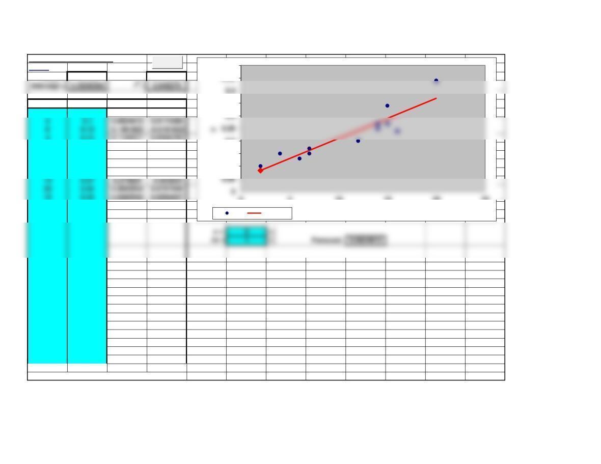
Example 9
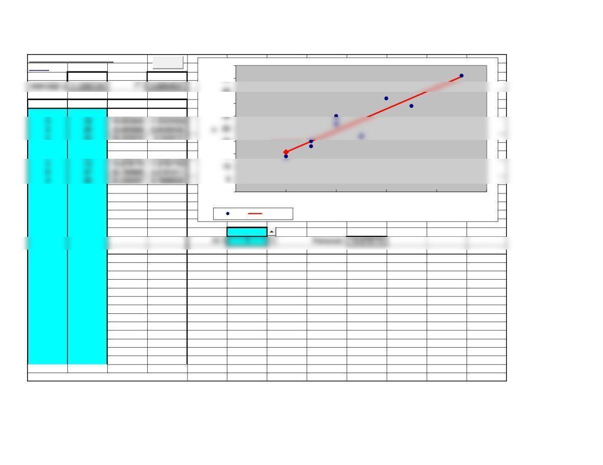
Simple Linear Regression
<Back
Slope = 0.0159 r = 0.9166657
x y Forecast Error
7 0.15 0.1621124 -0.0121124
2 0.1 0.0824612 0.0175388
6 0.13 0.1461822 -0.0161822
4 0.15 0.1143217 0.0356783
14 0.25 0.273624 -0.023624
15 0.27 0.2895543 -0.0195543
16 0.24 0.3054845 -0.0654845
12 0.2 0.2417636 -0.0417636
14 0.27 0.273624 -0.003624
20 0.44 0.3692054 0.0707946
15 0.34 0.2895543 0.0504457
7 0.17 0.1621124 0.0078876
Note: rows deleted from template for this example.
0.08246124
0.1
0.15
0.2
0.35
0.45
0.5
0 5 10 15 20 25
X
y Forecast
Clear
Page 81
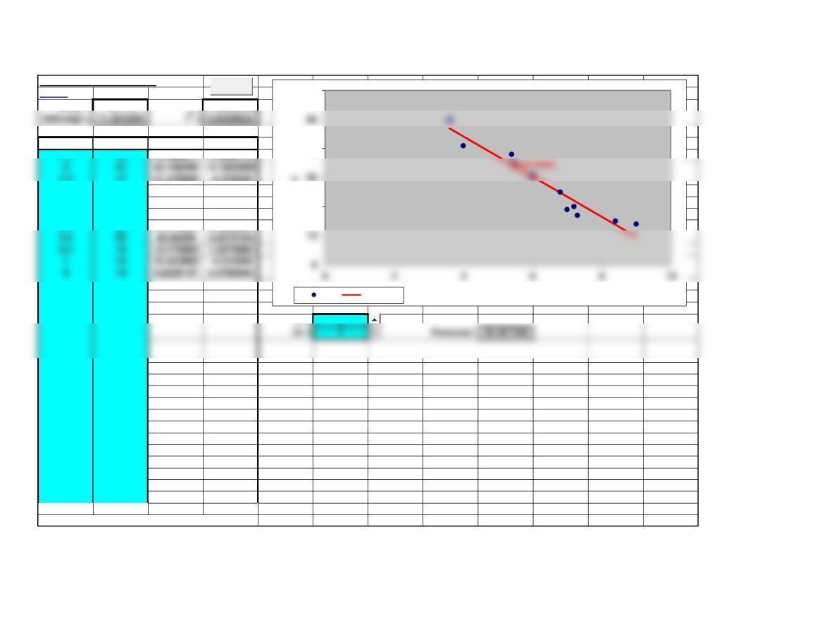
Example 10
Simple Linear Regression
<Back
Slope = -6.9145 r = -0.9658583
x y Forecast Error
7.2 20 22.069974 -2.0699737
441 44.196299 -3.1962989
7.3 17 21.378526 -4.378526
5.5 35 33.824584 1.1754161
6.8 25 24.835764 0.1642357
631 30.367346 0.6326544
5.4 38 34.516032 3.4839684
3.6 50 46.96209 3.0379104
8.4 15 13.772602 1.2273983
719 23.452869 -4.452869
914 9.6239157 4.3760843
x = 6
Note: rows deleted from template for this example.
20
40
60
Y
X
y Forecast
Clear
Page 82
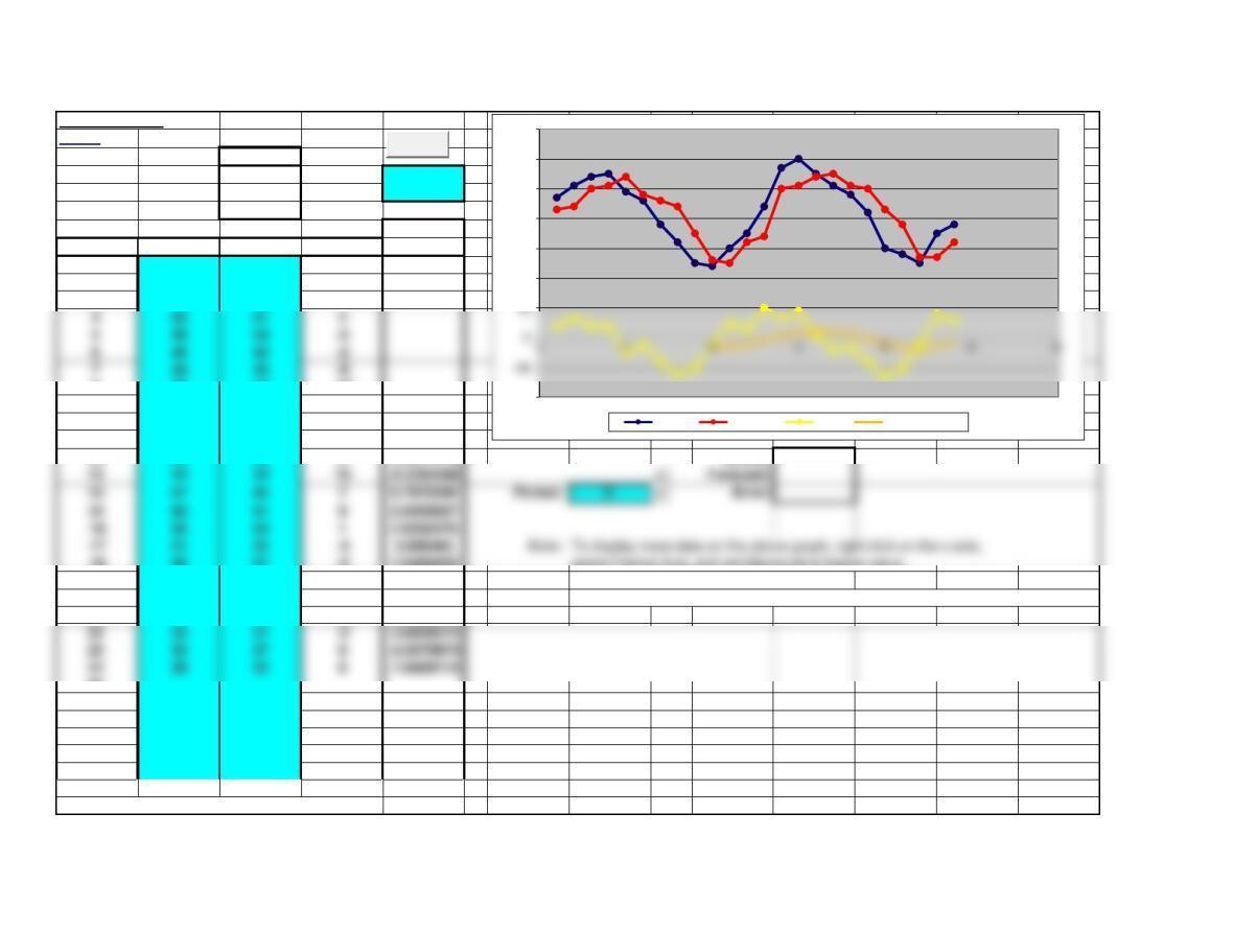
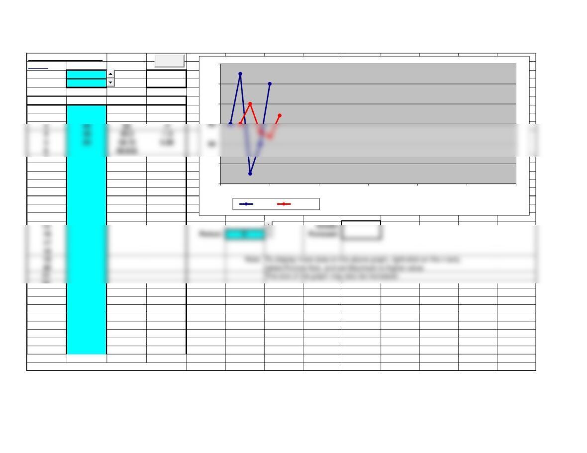
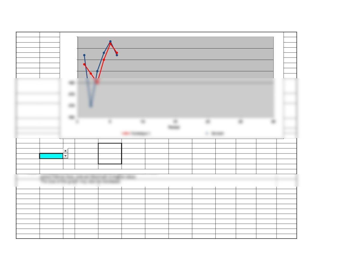
Example 12
Tracking Signal
<Back
Forecast
MAD = 6.125 Initial = 10
MSE = 50.652174 a = 0.2
MAPE = 16.43%
Tracking
Period Actual Forecast Error Signal
147 43 4#N/A
251 44 7#N/A
354 50 4#N/A
832 44 -12 #N/A
925 35 -10 #N/A
10 24 26 -2 -3.4482759
11 30 25 5 -2.6595745
12 35 32 3 -2.3474178 Actual: #N/A
14 57 50 7 0.7972346 Period: 0 Error: #N/A
15 60 51 9 2.0535857
16 55 54 1 2.6530476
17 51 55 -4 2.066465 Note: To display more data on the above graph, right click on the x-axis,
18 48 51 -3 1.6466055 select Format Axis, and set Maximum to higher value.
19 42 50 -8 0
The size of the graph may also be increased.
20 30 43 -13 -1.8599521 The range of the y-axis may also be adjusted to better view the tracking signal.
21 28 38 -10 -3.0296876
22 25 27 -2 -3.8620575
23 35 27 8 -2.5078974
24 38 32 6 -1.6609115
25 #N/A #N/A
26 #N/A #N/A
27 #N/A #N/A
28 #N/A #N/A
29 #N/A #N/A
30 #N/A #N/A
Note: rows deleted from template for this example.
-20
20
30
40
50
60
70
Period
Actual Forecast Error Tracking Signal
Clear
Page 83
455 51 4#N/A
549 54 -5 #N/A
646 48 -2 #N/A
738 46 -8 #N/A
Solved Problem 1b
Moving Average
<Back
MAD = 3.33
Periods = 3 MSE = 25.78
Period Actual Forecast Error
160 #N/A
265 #N/A
659
7#N/A
8#N/A
9#N/A
10 #N/A
11 #N/A
12 #N/A
13 #N/A
14 #N/A
15 #N/A Actual: #N/A
16 #N/A Period: 0 Forecast: #N/A
17 #N/A
18 #N/A
19 #N/A Note: To display more data on the above graph, right click on the x-axis,
20 #N/A select Format Axis, and set Maximum to higher value.
21 #N/A The size of the graph may also be increased.
22 #N/A
23 #N/A
24 #N/A
25 #N/A
26 #N/A
27 #N/A
28 #N/A
29 #N/A
30 #N/A
Note: rows deleted from template for this example.
56
62
64
66
Clear
Page 84
355 #N/A
458 60 -2
564 59.333333 4.6666667
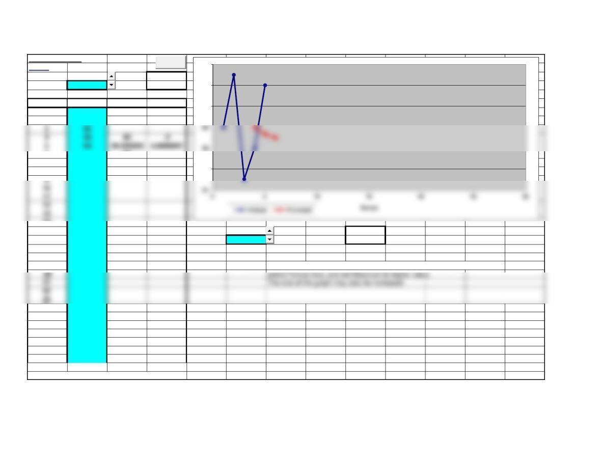
Solved Problem 1d
Exponential Smoothing
<Back
a = 0.4 MAD = 4.62
Da = 0.1 MSE = 34.44
Period Actual Forecast Error
160 #N/A
265 60 5
7#N/A
8#N/A
9#N/A
10 #N/A
11 #N/A
12 #N/A
13 #N/A
14 #N/A
15 #N/A Actual: #N/A
21 #N/A The size of the graph may also be increased.
22 #N/A
23 #N/A
24 #N/A
25 #N/A
26 #N/A
27 #N/A
28 #N/A
29 #N/A
30 #N/A
Note: rows deleted from template for this example.
54
56
62
64
66
0 5 10 15 20 25 30
Period
Actual Forecast
Clear
Page 85
355 62 -7
458 59.2 -1.2
564 58.72 5.28
Trend and Seasonal
<Back Slope = 3
Intercept = 402
Number of “seasons” = 12
Season Index
Feb 1.3
Mar 1.3
Aug 0.6
Sep 0.7
Oct 1
Period Season Trend Index Forecast Trend: #N/A
1 Feb 405 1.3 526.5 Index: #N/A
2 Mar 408 1.3 530.4 Period: 0 Forecast: #N/A
3 Apr 411 1.1 452.1
13 Feb 441 1.3 573.3
14 Mar 444 1.3 577.2
15 Apr 447 1.1 491.7
16 May 450 0.8 360
17 Jun 453 0.7 317.1
18 Jul 456 0.8 364.8
100
400
500
600
700

22 Nov 468 1.1 514.8
23 Dec 471 1.4 659.4
24 Jan 474 1.2 568.8
25 Feb 477 1.3 620.1
26 Mar 480 1.3 624
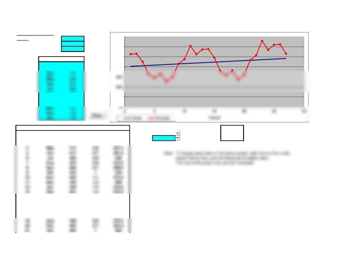
Solved Problem 3
Linear Trend Equation
<Back
Slope = 1.7500 MAD = 1.86
Intercept = 45.472222 MSE = 5.23
Period Actual Forecast Error
144 47.222222 -3.2222222 1
252 48.972222 3.0277778 2
555 54.222222 0.7777778 5
655 55.972222 -0.9722222 6
760 57.722222 2.2777778 7
856 59.472222 -3.4722222 8
962 61.222222 0.7777778 9
14 69.972222
15 #N/A Actual: #N/A
16 #N/A Period: 0 Forecast: #N/A
17 #N/A
18 #N/A
19 #N/A Note: To display more data on the above graph, right click on the x-axis,
20 #N/A select Format Axis and set Maximum to higher value.
21 #N/A The size of the graph may also be increased.
22 #N/A
23 #N/A
24 #N/A
25 #N/A
26 #N/A
27 #N/A
28 #N/A
29 #N/A
30 #N/A
Note: rows deleted from template for this example.
10
20
50
60
70
80
Clear
Page 88
350 50.722222 -0.7222222 3
454 52.472222 1.5277778 4
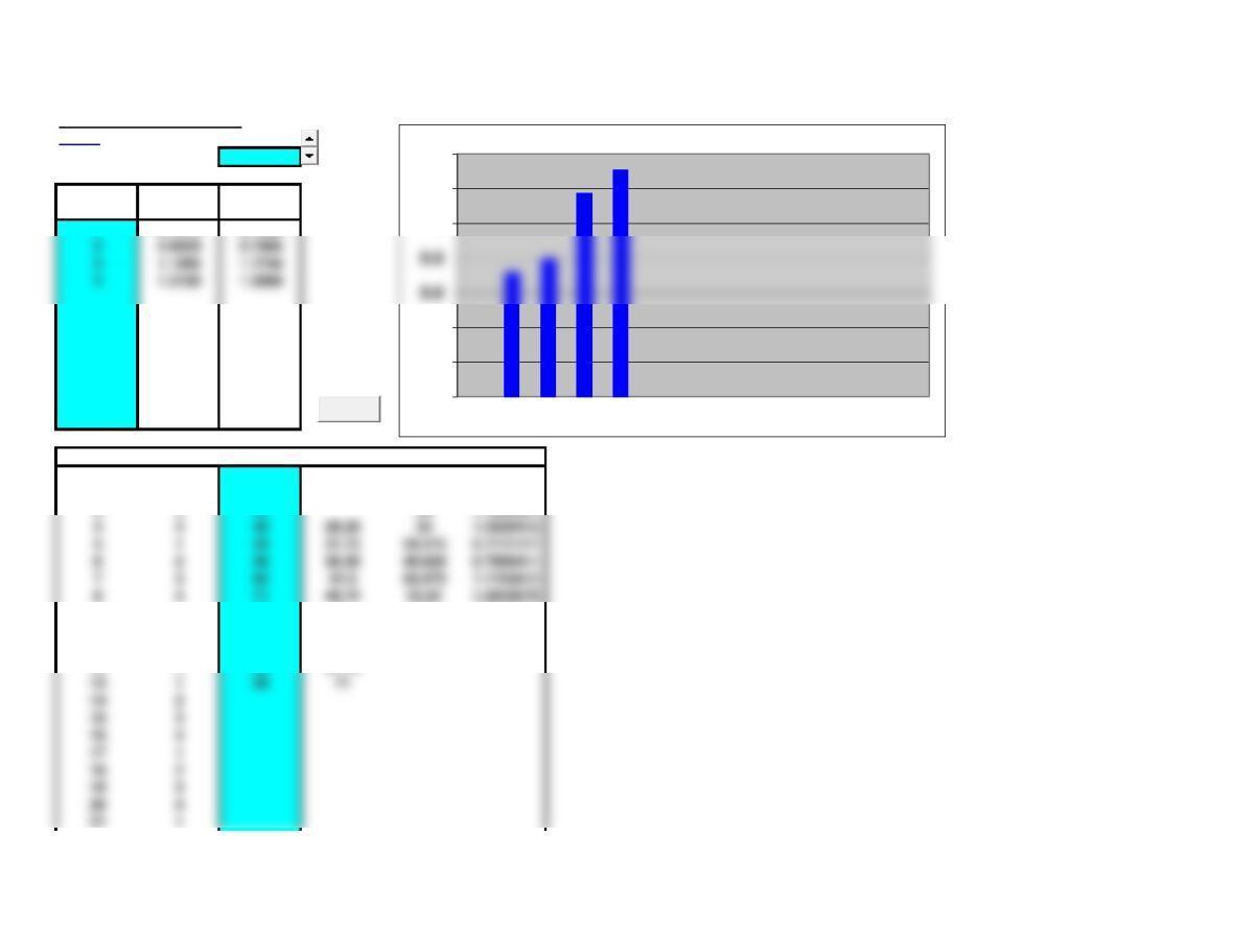
Compute Seasonal Indexes
<Back
Number of “seasons” = 4
Season Average Standard
Index Index
1 0.7275 0.7206 season season
3 0
season season
4 0
season season
0 0
season season
0 0
Period Season Actual MA Center Index
1 1 14 #N/A #N/A
2 2 18 #N/A #N/A
3 3 35 #N/A 30 1.1666667
4 4 46 28.25 34 1.3529412
5 1 28 31.75 39.375 0.7111111
6 2 36 36.25 45.625 0.7890411
7 3 60 42.5 50.875 1.1793612
8 4 71 48.75 55.25 1.2850679
9 1 45 53 60.5 0.7438017
10 254 57.5 65.625 0.8228571
11 384 63.5 69.375 1.2108108
12 488 67.75 #N/A
13 158 71 #N/A
14 2#N/A #N/A
15 3#N/A #N/A
16 4#N/A #N/A
17 1#N/A #N/A
18 2#N/A #N/A
19 3#N/A #N/A
0
0.2
0.4
1
1.2
1.4
1
2
3
4
Clear
2 0.8059 0.7984 1 0
3 1.1856 1.1744 season season
4 1.3190 1.3066 2 0
season season

22 2#N/A #N/A
23 3#N/A #N/A
24 4#N/A #N/A
25 1#N/A #N/A
26 2#N/A #N/A
27 3#N/A #N/A
28 4#N/A #N/A
29 1#N/A #N/A
30 2#N/A #N/A
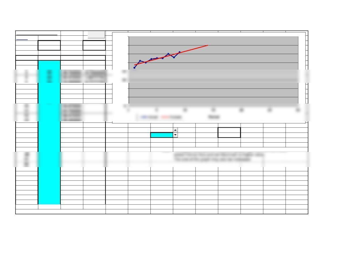
Solved Problem 6
Simple Linear Regression
<Back
Slope = 4.2753 r = 0.9276226
x y Forecast Error
946 45.606742 0.3932584
318 19.955056 -1.9550562
320 19.955056 0.0449438
522 28.505618 -6.505618
427 24.230337 2.7696629
734 37.05618 -3.0561798
214 15.679775 -1.6797753
637 32.780899 4.2191011
430 24.230337 5.7696629
x = 2
Note: rows deleted from template for this example.
15.67977528
0
15
20
35
40
45
50
0 2 4 6 8 10
X
y Forecast
Clear
Page 91

Solved Problem 7
Forecast Accuracy Notes
<Back
Technique 1 Technique 2
MSE = 49.6 MSE = 52.8 MSE =
MAPE = 0.9725% MAPE = 1.1714% MAPE =
Period Actual Technique 1 Error % Error Technique 2 Error % Error
1492 488 4 0.81% 495 -3 -0.61%
2470 484 -14 -2.98% 482 -12 -2.55%
3485 480 5 1.03% 478 7 1.44%
4493 490 3 0.61% 488 5 1.01%
5498 497 1 0.20% 492 6 1.20%
6492 493 -1 -0.20% 493 -1 -0.20%
7
8
9
10
11
12
13
14
15
16
17
18
21
22
23
24
25
26
27
28
29
30
31
32
33
Clear
Page 92

Solved Problem 7
34
35
36
37
48
49
50
51
52
53
54
55
56
57
58
59
60
61
62
63
64
65
66
67
68
69
70
71
72
73
74
Page 93
38
39
40
41
42
43
44
45
46
47
Solved Problem 7
75
76
77
78
89
90
91
92
93
94
95
96
97
98
99
100
101
102
103
104
105
106
107
108
109
110
111
112
113
114
115
Page 94
79
80
81
82
83
84
85
86
87
88
Solved Problem 7
116
117
118
119
130
131
132
133
134
135
136
137
138
139
140
141
142
143
144
145
146
147
148
149
150
151
152
153
154
155
156
Page 95
120
121
122
123
124
125
126
127
128
129
Solved Problem 7
157
158
159
160
171
172
173
174
175
176
177
178
179
180
181
182
183
184
185
186
187
188
189
190
191
192
193
194
195
196
197
Page 96
161
162
163
164
165
166
167
168
169
170

Solved Problem 7
198
199
200
201
212
213
214
215
216
217
218
219
220
221
222
223
224
225
226
227
228
229
230
231
232
233
234
235
236
237
238
Page 97
202
203
204
205
206
207
208
209
210
211

Solved Problem 7
239
240
241
242
243
244
245
246
247
248
249
250
Notes: You can Copy the forecasts from another template and Paste Special Values into this template.
Page 98
Solved Problem 7
Actual: #N/A
Forecast 1: #N/A
Period: 0 Forecast 2: #N/A
Forecast 3: #N/A
Note: To display more data on the above graph, right click on the x-axis,
485
490
495
500
Page 99

Chapter 3 – Problems 1-7 Note: This worksheet displays results only, you must copy the shaded
<Back area into the corresponding template to make additional calculations.
2. Linear Trend Equation
Slope = 0.5000 MAD = 1.45
Intercept = 16.857143 MSE = 3.64
Period Actual Forecast Error
119 17.357143 1.6428571
218 17.857143 0.1428571
315 18.357143 -3.3571429
Moving Average
MAD = 2.70
Periods = 5 MSE = 17.96
Period Actual Forecast Error
119 #N/A
218 #N/A
315 #N/A
420 #N/A
518 #N/A
622 18 4
720 18.6 1.4
Exponential Smoothing
a = 0.2 MAD = 1.96
Da = 0.1 MSE = 6.74
Period Actual Forecast Error
119 #N/A
218 19 -1
315 18.8 -3.8
420 18.04 1.96
518 18.432 -0.432
622 18.3456 3.6544
720 19.07648 0.92352
819.261184
Exponential Smoothing (naive approach)
420 18.857143 1.1428571
622 19.857143 2.1428571
720 20.357143 -0.3571429
820.857143