Chapter 3
Probability Distributions
Learning Objectives
1. Understand the concepts of a random variable and a probability distribution.
2. Be able to distinguish between discrete and continuous random variables.
6. Understand the difference between how probabilities are computed for discrete and continuous
random variables.
7. Know how to compute probability values for a continuous uniform probability distribution and be
able to compute the expected value and variance for such a distribution.
Markov Processes
Solutions:
1. a. values: 0,1,2,…,20
discrete
d. values: 0 x 8
continuous
e. values: x 0
continuous
2. a. f (200) = 1 – f (-100) – f (0) – f (50) – f (100) – f (150)
= 1 – 0.95 = 0.05
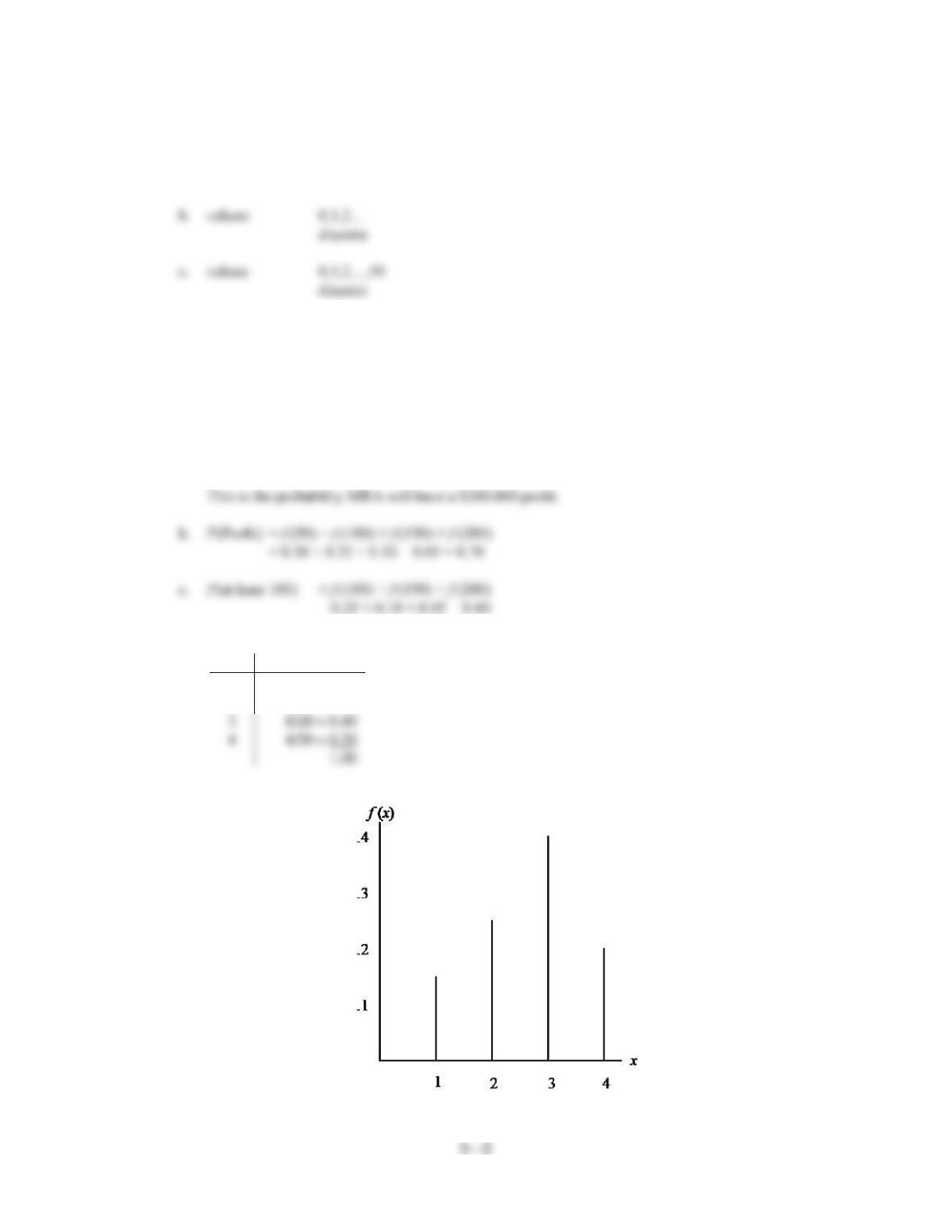
3. a.
x
f (x)
1
3/20 = 0.15
2
5/20 = 0.25
3
8/20 = 0.40
4
4/20 = 0.20
b.
Markov Processes
c. f (x) 0 for x = 1,2,3,4.
f (x) = 1
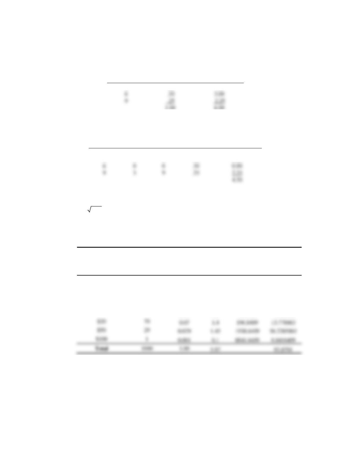
4. a.
x
f (x)
x f (x)
1.00
6.00
E (x) = = 6.00
b.
x
x –
(x –
)2
f (x)
(x –
)2 f (x)
4.50
Var (x) =
2 = 4.50
c.
4.50 2.12
==
5. Let X = amount of money in a randomly selected bar of soap.
The following table shows the calculations for parts (a) and (b).
Distribution of Paper
Currency Prizes
Bill
Denomination (x)
Number of
Bills
f(x)
xf(x)
(x–
)2
(x–
)2f(x)
$1
520
0.52
0.52
24.7009
12.844468
$5
260
0.26
1.3
0.9409
0.244634
$10
120
0.12
1.2
16.2409
1.948908
$20
0.07
1.4
13.778863
$50
0.029
1.45
0.001
0.1
8.8416409
5.97
93.8791
a. E[X] = 5.97
b. St. Dev. (X) =
= 9.69
Chapter 17
c. Let Y = number of bars that contain a $50 or $100 bill. Observe that Y is a binomial random variable,
where n = numbers of bars purchased and p = probability of a bar containing a $50 or $100 bill =
(29/1000) + (1/1000) = .03. E[Y] = n × p = n × 0.03 = 3, thus n = 100. The customer needs to buy 100
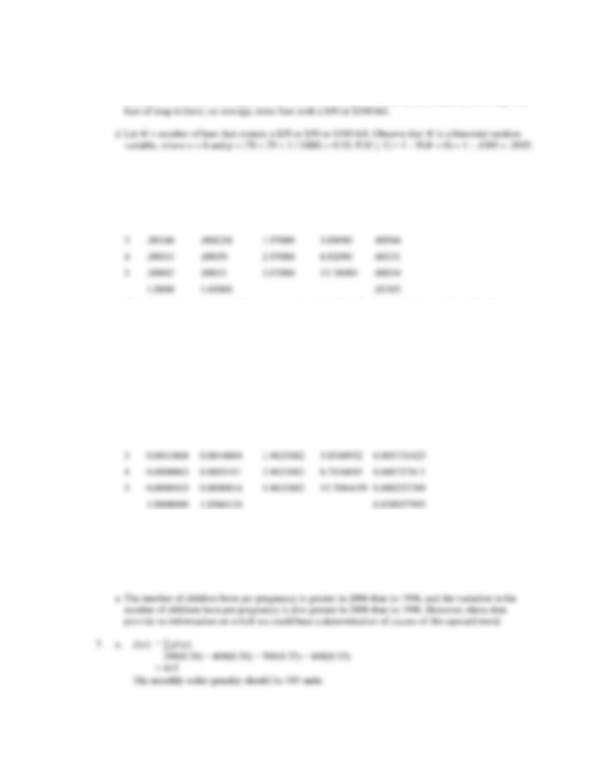
6. The following table shows the calculations for parts (a) and (b).
x f(x) xf(x) x-
(x-
)2 (x-
)2f(x)
1 .97176 .97176 -.03000 .00090 .00087
2 .026675 .05333 .97000 .94090 .02509
If we let x = 5 represent quintuplets or more, the probability distribution of the number children born per
pregnancy in 1996 is provided in the first two columns of the table above.
a. The expected value of the number children born per pregnancy in 1996 is E[x] = 1.030.
b. The variance of the number children born per pregnancy in 1996 is V[x] =
2 = 0.0331.
The following table shows the calculations for parts (c) and (d).
y f(y) yf(y) y-
(y-
)2 (y-
)2f(y)
1 0.965964 0.9650964 -0.0366118 0.0013404 0.001293639
2 0.0333143 0.0666286 0.9633882 0.9281168 0.030919551
If we let y = 5 represent quintuplets or more, the probability distribution of the number children born per
pregnancy in 2006 is provided in the first two columns of the table above.
c. The expected value of the number children born per pregnancy in 2006 is E[y] = 1.030.
d. The variance of the number children born per pregnancy in 2006 (after rounding) is V[y] =
2 = 0.0390.
Markov Processes
b. Cost: 445 @ $50 = $22,250
Revenue: 300 @ $70 = 21,000
$ 1,250 Loss
c.
x
f (x)
(x – µ)
(x – µ)2
(x – µ)2f (x)
300
0.20
–145
21025
4205.00
400
0.30
– 45
2025
607.50
500
0.35
3025
1058.75
600
0.15
24025
3603.75
8. a.
Medium:
E(x)
= xf (x)
= 50(0.20) + 150(0.50) + 200(3.0) = 145
Large:
E(x)
= xf (x)
= 0(0.20) + 100(0.50) + 300(0.30) = 140
Medium preferred.
b. Medium
x
f (x)
(x – µ)
(x – µ)2
(x – µ)2f (x)
50
0.20
–95
9025
1805.0
150
0.50
200
0.30
3025
2 = 2725.0
Large
x
f (x)
(x – µ)
(x – µ)2
(x – µ)2f (x)
0
0.20
–140
19600
3920
100
0.50
300
0.30
25600
2 = 12,400
Medium preferred due to less variance.
9. a.
11
22!
(1) (0.4) (0.6) (0.4)(0.6) 0.48
11!1!
f
= = =
b.
02
22!
(0) (0.4) (0.6) (1)(0.36) 0.36
00!2!
f
= = =
= = =
Chapter 17
e. E (x) = n p = 2 (.4) = .8
10. a. f (0) = .3487
b. f (2) = .1937
0.9 0.9487
==
11. a. In a sample of six British citizens, the probability that two believe inequality is too large is
( ) ( ) ( )
0375.74.1.74
2
6
2262 =−
=−
f
b. In a sample of six British citizens, the probability that at least two believe inequality is too large is
( ) ( ) ( ) ( ) ( ) ( )
( ) ( ) ( ) ( ) ( ) ( )
74.1.74
4
6
74.1.74
3
6
74.1.74
2
6
654322
464363262
−
+−
+−
=
++++=
−−−
fffffleastatP
c. In a sample of four British citizens, the probability that none believe inequality is too large is
( ) ( ) ( )
0046.74.1.74
0
4
0040 =−
=−
f
12. a. Probability of a defective part being produced must be .03 for each trial; trials must be independent.
Markov Processes
c. P (no defects) = (.97) (.97) = .9409
13. a. 0.90
b. P(at least 1) = f (1) + f (2)
f (1) =
11
2! (0.9) (0.1)
1!1!
= 2 (0.9) (0.1) = 0.18
Therefore P(at least 1) = 0.18 + 0.81 = 0.99
Alternatively
c. P(at least 1) = 1 – f (0)
f (0) =
03
3! (0.9) (0.1) 0.001
0!3! =
Therefore P(at least 1)= 1 – 0.001 = 0.999
14. a.
2
2
() !
xe
fx x
−
=
b.
= 6 for 3 time periods
Chapter 17
e.
66
6
(6) 0.1606
6!
e
f−
==
f.
54
4
(5) 0.1563
5!
e
f−
==
15. a.
= 48 (5 / 60) = 4
34
4 (64)(0.0183)
(3) 0.1952
3! 6
e
f−
= = =
The probability none will be waiting after 5 minutes is .0183.
d.
= 48 (3 / 60) = 2.4
0 2.4
2.4
(0) 0.0907
0!
e
f−
==
The probability of no interruptions in 3 minutes is .0907.
16. a.
07 7
7
(0) .0009
0!
e
fe
−−
= = =
b. probability = 1 – [f(0) + f(1)]
17 7
7
(1) 7 .0064
1!
e
fe
−−
= = =
Markov Processes
d. probability = 1 – [f(0) + f(1) + f(2) + f(3) + f(4)]
= 1 – [.0009 + .0064 + .0223 + .0521 + .0912]
= .8271
Note: Appendix B was used to compute the Poisson probabilities f(0), f(1), f(2), f(3) and f(4) in
part (d).
17. a.
0 10 10
10
(0) 0.000045
0!
e
fe
−−
= = =
Similarly, f (2) = 0.00225, f (3) = 0.0075
Therefore f (0) + f (1) + f (2) + f (3) = 0.010245
c. 15 second period, therefore we have 2.5 arrivals/15 second period
18. a.
b. P(x = 1.25) = 0. the probability of any single point is zero since the area under the curve above any
single point is zero.
1
2
3
.50 1.0 1.5 2.0
f (x)
x
Chapter 17
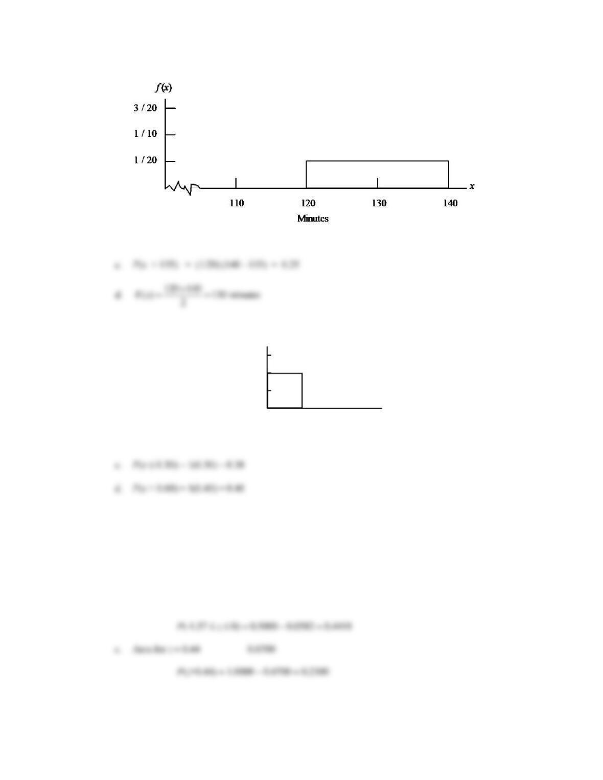
19. a.
b. P(x 130) = (1/20) (130 – 120) = 0.50
20. a.
b. P(0.25 < x < 0.75) = 1(0.50) = 0.50
21. a. Area for z = 0 0.5000
Area for z = 0.83 0.7967
P(0 z 0.83) = 0.7967 – 0.5000 = 0.2967
b. Area for z = -1.57 0.0582
Area for z = 0 0.5000
.5
1.0
1.5
1 2 3
f (x)
x
0
Markov Processes
d. Area for z = -0.23 0.4090
P(z -0.23) = 1.0000 – 0.4090 = 0.5910
22. a. Area = 0.9750 z = 1.96
b. Area for z = 0 0.5000
Area for z must be 0.5000 + 0.4750 = 0.9750 z = 1.96
c. Area = 0.7291 z = 0.61
23. a. Area = 0.2119 z = -0.80
b. Area outside the interval = 1.0000 – 0.9030 = 0.0970 must be split between the two tails.
Cumulative probability at z must be 0.5(0.0970) + 0.9030 = 0.9515 z = 1.66
c. Area outside the interval = 1.0000 – 0.2052 = 0.7948 must be split between the two tails.
24. a. At x = 180
180 200 0.50
40
z−
= = −
Cumulative probability = 0.3085
Chapter 17
b. At x = 250
250 200 1.25
40
z−
==
c. At x = 100
100 200 2.50
40
z−
= = −
Cumulative probability = 0.0062
P(x 100) = 0.0062
Cumulative probability = 0.7341
P(225 x 250) = 0.8944 – 0.7341 = 0.1603
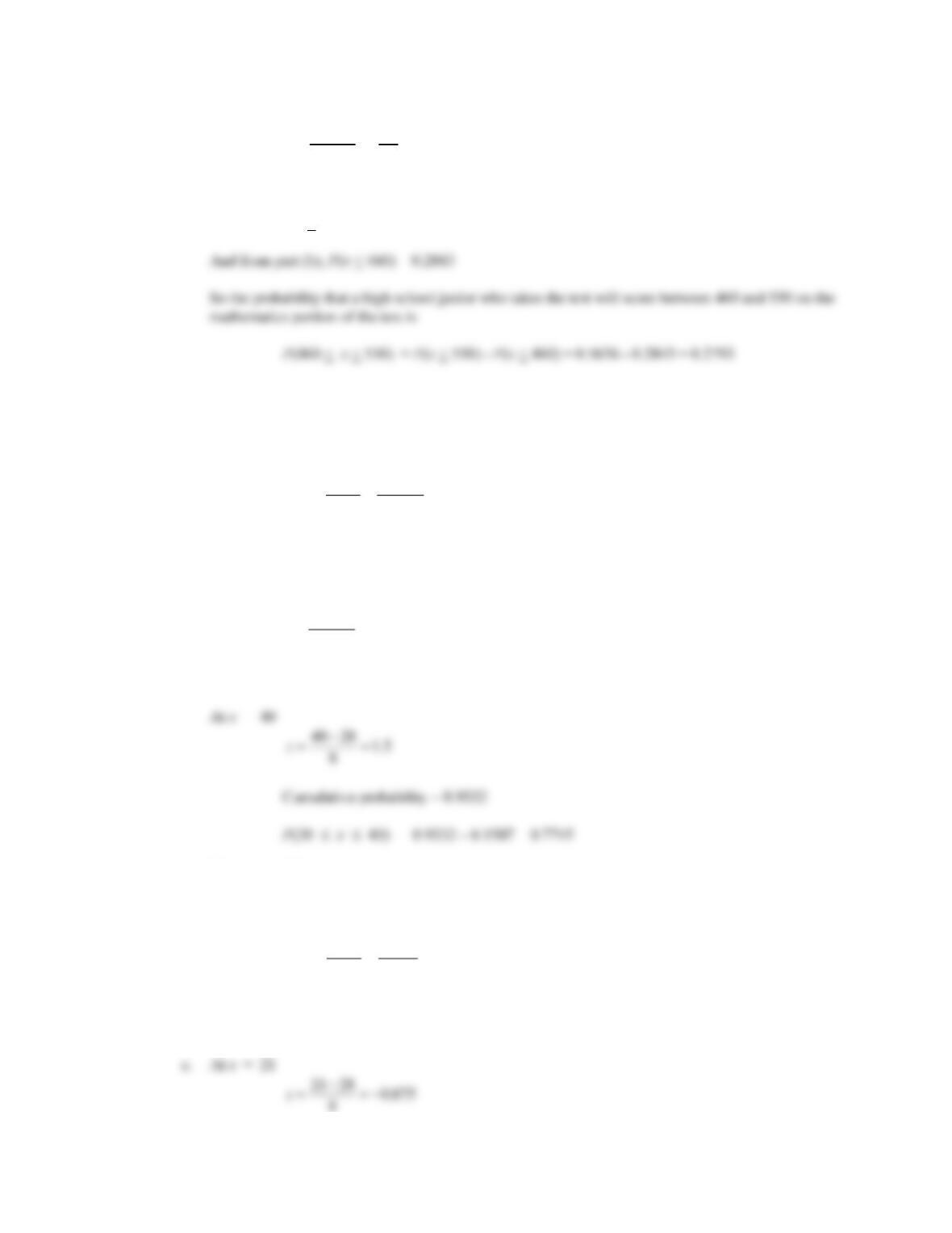
25. a. At x = 610
610 530 80 0.65
123 123
z−
= = =
Cumulative probability = 0. 7422
P(x 610) = 1.0000 – 0. 7422 = 0.2578
b. At x = 460
460 530 70 .57
123 123
z−−
= = = −
Markov Processes
c. At x = 550
𝑧 = 550−530
123 = 20
123 = .16
Cumulative probability = 0.5636
P(x < 530) = 0.5636
d. The highest 10% of the scores on the mathematics portion of the test would be in the upper tail of the
normal distribution with a cumulative probability 0.90. From the table of the cumulative standard
normal distribution, the area or probability closest to 0.90 is 0.8997. The corresponding z = 1.28. Thus
we have.
530
1.28 123
xx
−−
==
Therefore solving for x, we have x = 123(1.28) + 530 = 687.44. The top 10% of the scores on the
mathematics portion of the test will be 687 or higher.
26. a. At x = 20
20 28 1.0
8
z−
= = −
Cumulative probability = 0.1587
b. The oldest 15% of the accounts would be in the upper tail of the normal distribution with a cumulative
probability 0.85. The area or probability closest to 0.85 occurs for the cumulative probability of 0.8508.
The corresponding z = 1.04. Thus we have.
28
1.04 8
xx
−−
==
Therefore solving for x, we have x = 8(1.04) + 28 = 36.32. An account should be sent a reminder
letter after 36.32 days.
Chapter 17
Cumulative probability = 0.1906
Therefore 0.1906 or approximately 19% of the accounts will receive the discount.
27. Let Y = inches of snowfall on December 24 through 28. Y is a normal random variable with mean of 6
inches and standard deviation of 0.559 inches.
= 0.6
For a cumulative probability of 0.02, z = -2.05.
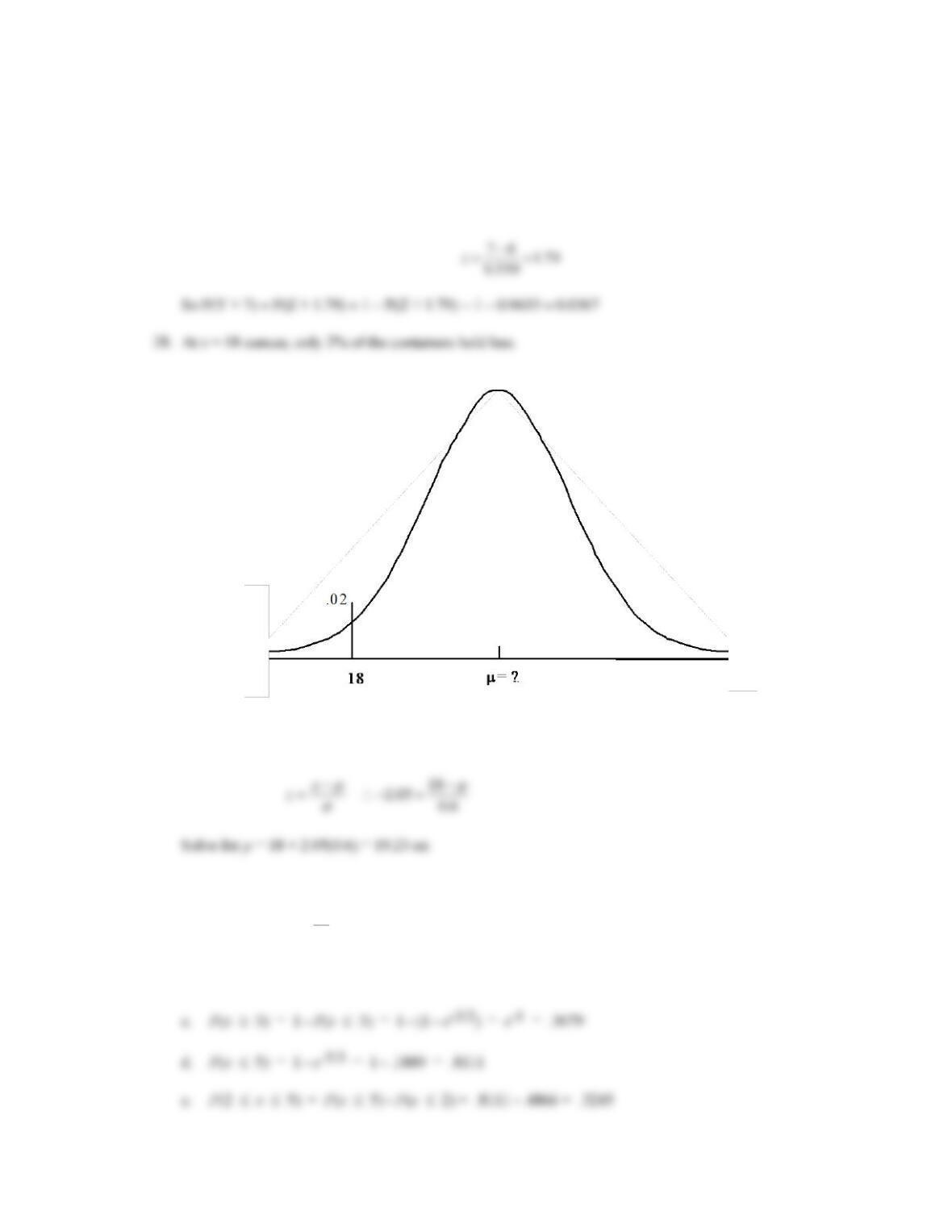
The mean filling weight must be 19.23 ounces if only 2% are filled with less than 18 ounces.
29. a.
0
3
0
( ) 1
x
P x x e
−
= −
b. P(x 2) = 1 – e-2/3 = 1 – .5134 = .4866
Markov Processes
30. a. P(x 2) = 1 – e-2/2.3 = .5809
b. P(x 3) = 1 – P(x 3) = 1 – (1 – e-3/2.3 ) = e-3/2.3 = .2713
31. a.
.04
.05
.06
.07
.08
.09
f
(
x
)
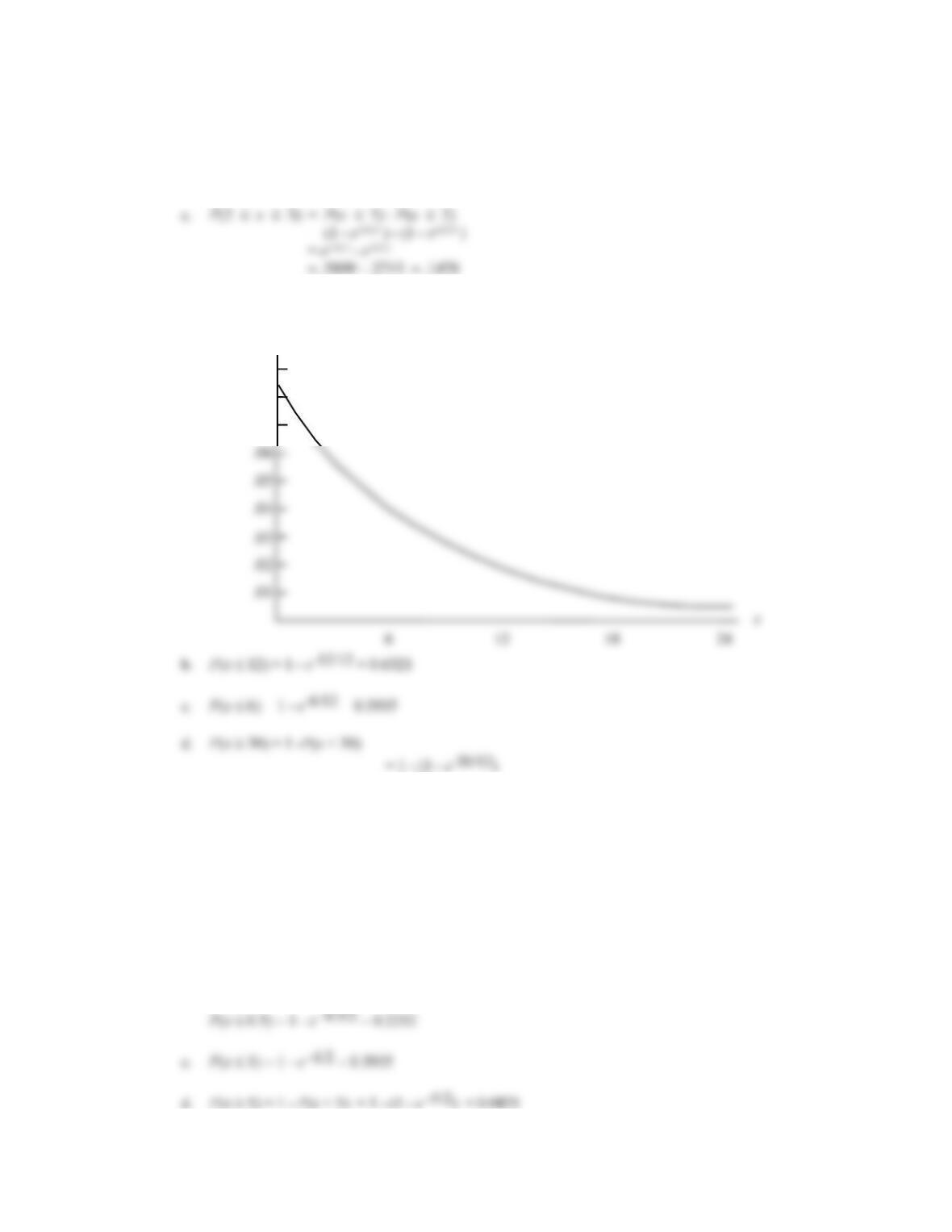
= 0.0821
32. a. 50 hours
b. P(x 25) = 1 – e–25/50 = 0.3935
c. P(x 100) = 1 -(1 – e-100/50) = 0.1353
33. a. 1/µ = 0.5 therefore µ = 2 minutes
b. Note: 30 seconds = 0.5 minutes
Chapter 17
34. a. P(x 2) = 1 – e-2/2.78 = .5130
b. P(x 5) = 1 – P(x 5) = 1 – (1 – e-5/2.78 ) = e-5/2.78 = .1655