
Chapter 03 – Forecasting
3-1
CHAPTER 03
FORECASTING
Forecasting is placed early in the text mainly because it is a point of departure. Some instructors like to
emphasize the operations part of operations management and de-emphasize the design part. Other
instructors prefer to blend the two. However, forecasting is an important input for both, and for that
reason, it is presented as early as possible.
Teaching Notes
This is a fairly long chapter, so you may want to be selective about the topics covered in order to shorten
the time devoted to it. I tend to devote more time to the time series methods than I do to regression
analysis, for several reasons. One is that students often are exposed to regression in their stat course(s).
I try to emphasize an intuitive approach to forecasting, with frequent reference to the importance of
plotting the data to assist the decision-maker in determining which forecasting technique may be more
appropriate to use.
In operations management, we forecast a wide range of future events, which could significantly affect the
long-term success of the firm. Most often the basic need for forecasting arises in estimating customer
demand for a firm’s products and services. However, we may need aggregate estimates of demand as well
as estimates for individual products. In most cases, a firm will need a long-term estimate of overall
Answers to Discussion and Review Questions
1. It depends on the situation at hand. In certain situations, one approach will be superior to the
other.
Quantitative techniques lend themselves to computerization, they are less subject to personal

Chapter 03 – Forecasting
3-2
2. Poor forecasting leads to poor planning. This could result in offering products and services
3. a. Consumer surveys may be invalid if they are not carefully constructed, administered, and
interpreted. Moreover, respondents may be ill-informed or otherwise formulate answers
which do not correctly reflect their future actions.
4. The delphi technique involves using a series of anonymous questionnaires, which are circulated
5. Control limits reveal the bounds of random errors; they enable managers to judge if a forecasting
technique is performing as well as it might (and hence, when a technique should be reevaluated).
6. The relative costs of reevaluating a forecast when nothing is wrong versus not reevaluating it
8. Exponential smoothing: requires less data storage, gives more weight to recent data, and is easier
to change responsiveness.
10. The choice of alpha in exponential smoothing depends on how responsive a forecast the manager
Chapter 03 – Forecasting
3-3
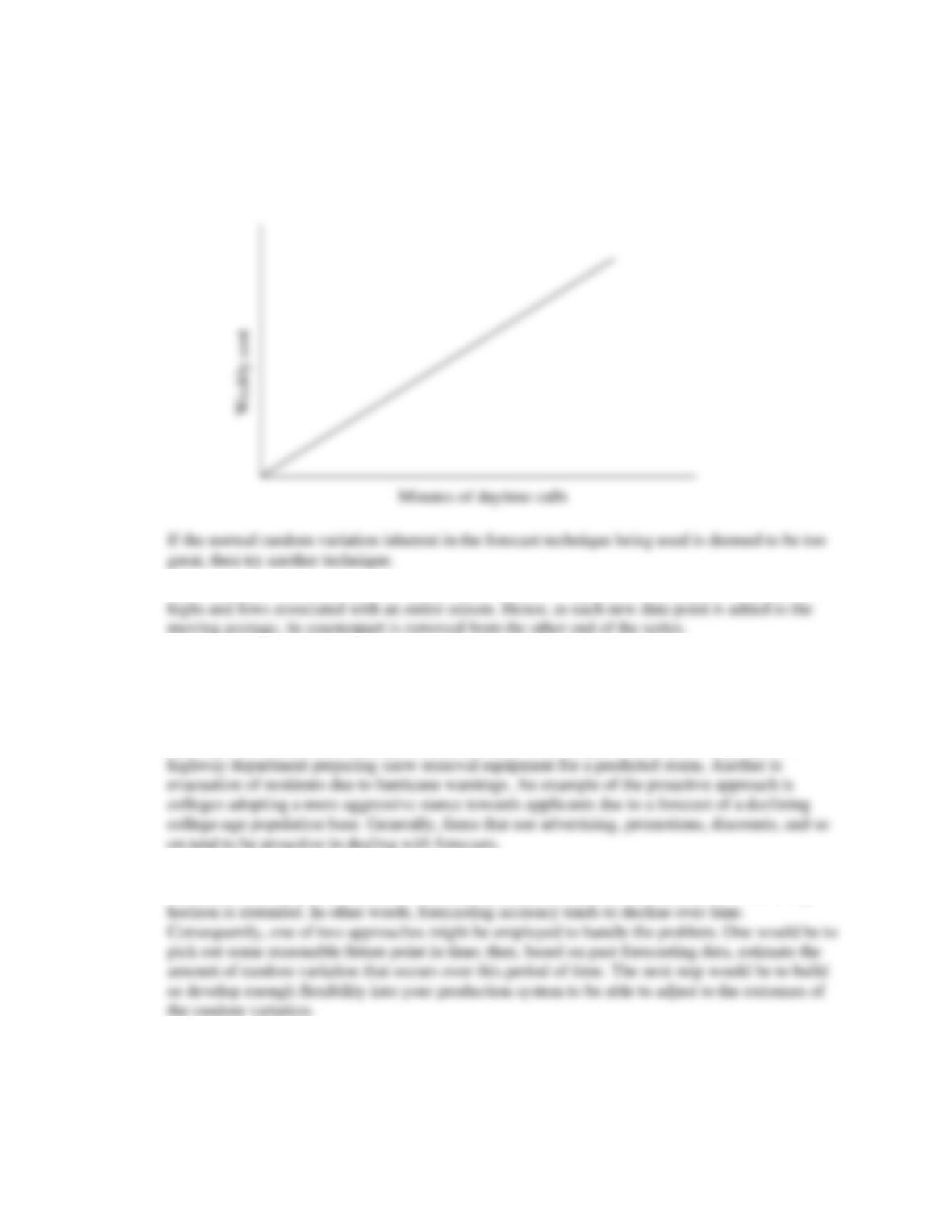
11. Of course the accuracy of your five-day weather forecast will depend on a number of variables
such as time of year, where you live, etc. But there is one trend that will establish itself and that is
as time passes from the first day to the fifth day, the accuracy of the forecast will decline. The
amount of random variation about the forecast (actual vs. forecast) would increase over time
somewhat like the following:
12. Each average is based on 12 months (four quarters, seven days, etc.), and therefore includes the
13. Sales indicate how much customers bought, while demand indicates how much they wanted. The
distinction is important when demand exceeds supply, because supply places an upper bound on
the data.
14. A reactive approach takes the forecast as a “given” while a proactive approach takes an
unacceptable forecast and attempts to alter demand. An example of the reactive approach is a
15. There is always going to be a certain amount of random variation about the forecast. The amount
of this random variation about the forecast (actual vs. forecast) will increase as the forecasting

Chapter 03 – Forecasting
3-4
16. Forecasting in the context of supply chain involves connection and communication between the
supply chain databases. For example, assume that Company X is a durable goods manufacturer.
Based on the market and historical sales information, Company X determines short and
17. It depends on the situation. Sometimes one approach is better, sometimes the other, and
sometimes both are used. Considerations include the importance of the forecasts, how quickly the
18. In forecasting initial sales for the new version of its software, the software producer should
consider:
a. The historical demand information for the old version.
b. The features of the new version of the software in comparison to the features of the old
version.
19.
a. Demand for Mother’s Day greeting cards: Naïve using last year’s demand.
b. Popularity of a new TV series: Delphi, or associative based on features of existing series.

Chapter 03 – Forecasting
3-5
Taking Stock
1. If the forecasts are too responsive and it becomes too sensitive to the changes in actual demand, it
2. Forecasting needs to be a collaborative effort involving marketing, production and technical
3. The technology had tremendous impact on forecasting mainly because of the advancement of the
computer technology. Computer technology plays a very important role in preparing forecasts
Critical Thinking Exercise
1. The conditions that would have to exist for driving a car that are analogous to the assumptions
made when using exponential smoothing are that the immediate future will be like the recent past.
This would suggest:
a. No sharp curves or turns on the road
2. Instantaneous re-supply and/or completely flexible capacity.
3. Potential investors would expect information on the current and future size of the market, the
4. How to handle a poor forecast (i.e., one that is substantially above or below actual demand)
would depend on what the items is, and on a number of factors. For example, a low forecast
would lead to a stockout. How critical that is would relate to how important that is the customers
5. Although understandable Omar’s approach is not ethical. He should turn in the forecast based on
the information he has and tell his superiors that he thinks he can get those numbers up.
6. Student answers will vary.
Chapter 03 – Forecasting
3-6
Memo Writing Exercises
1. If there are significant patterns in the forecast errors, it is possible to make improvements to
forecasts that fall within predetermined control limits. Checking for patterns in the data is usually
done by visual inspection. If a significant pattern is discovered, changes in the forecasting model
can be made to improve the accuracy of the forecasts. The possible changes may involve using a
Solutions
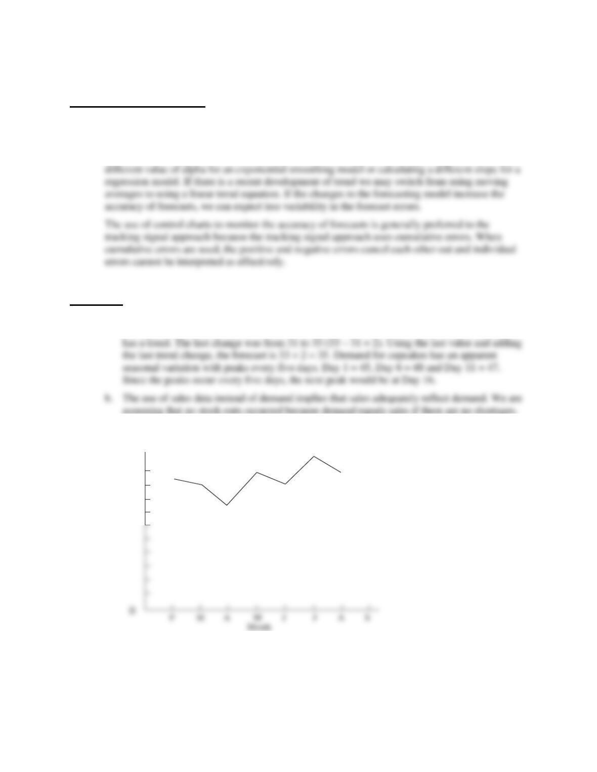
1. a. Plotting each data set reveals that blueberry muffin orders are stable, varying around an
average. Therefore, the naïve forecast is the last value, 33. The demand for cinnamon buns
2. a.
0
Sales
20
Chapter 03 – Forecasting
b. 1)
t
Y
tY
From Table 3–1 with n = 7, t = 28, t2 = 140
50.
)28(28)140(7
)132(28)542(7
)t(tn
YttYn
b22 =
−
−
=
−
−
=
5
18
90
6
22
132
7
20
140
1
19
19
2
18
36
3
15
45
2)
19
5
2022182015
MA5=
++++
=
3)
Month
Forecast =
F(old)
+
.20[Actual – F(old) ]
May
18.04 =
18.8
+
.20[ 15 – 18.8 ]
June
18.43 =
18.04
+
.20[ 20 – 18.04 ]
July
18.34 =
18.43
+
.20[ 18 – 18.43 ]
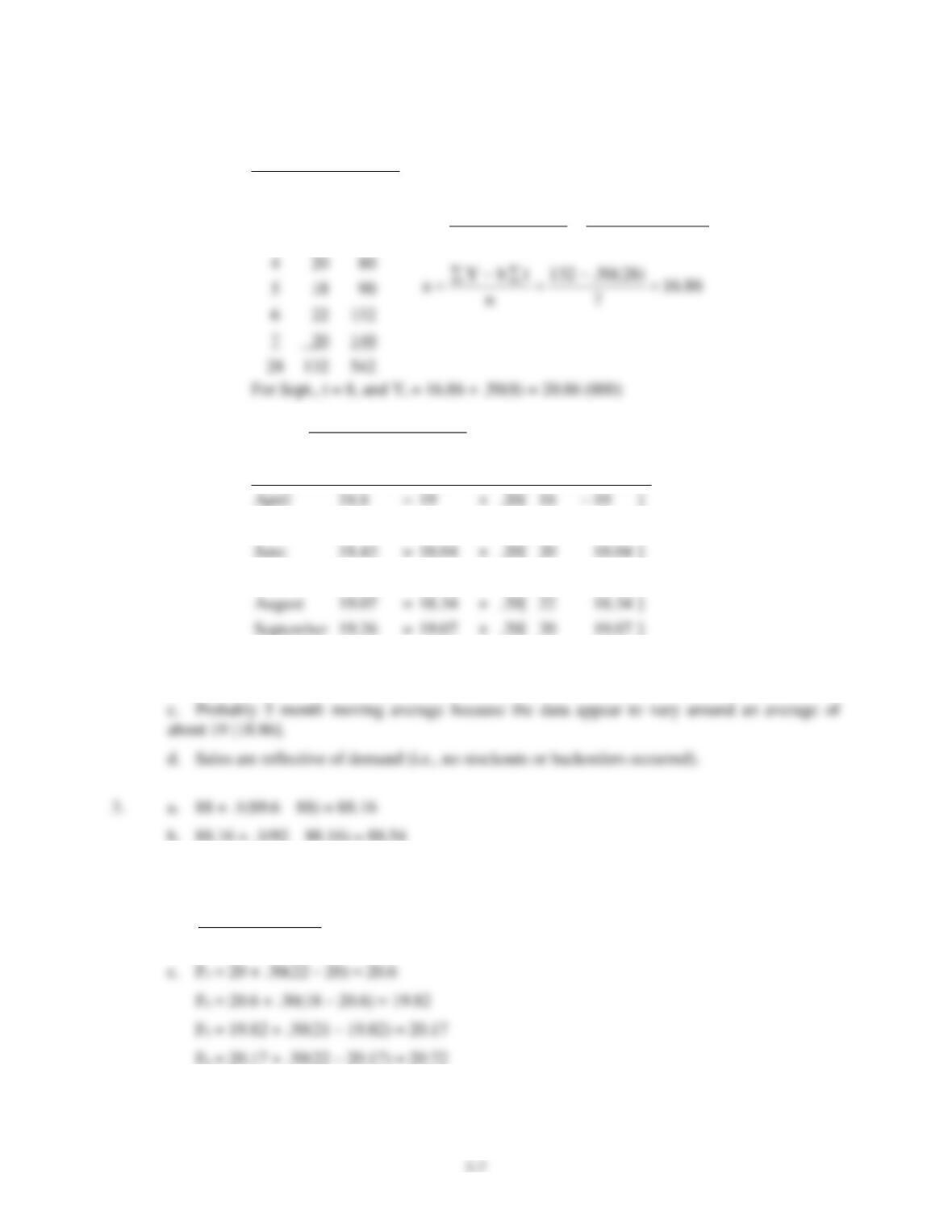
September
19.26 =
19.07
+
.20[ 20 – 19.07 ]
4) 20
5) .6 (20) + .3(22) + .1(18) = 20.4
4. a. 22
b.
75.20
4
22211822 =
+++

Chapter 03 – Forecasting
3-8
5. a. Annual sales are increasing by 15,000 bottles per year.
6.
t20500t
10
200
500Yt−=−=
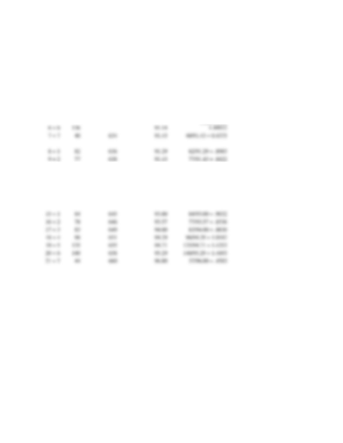
7.
a.
t
Y
t*Y
t2
1
220
220
1
2
245
490
4
3
280
840
9
4
275
1,100
16
5
300
25
6
310
1,860
36
7
350
2,450
49
8
360
64
9
400
3,600
81
380
3,800
420
4,620
460
5,980
475
6,650
500
7,500
510
525
8,925
541
9,738
Chapter 03 – Forecasting
2
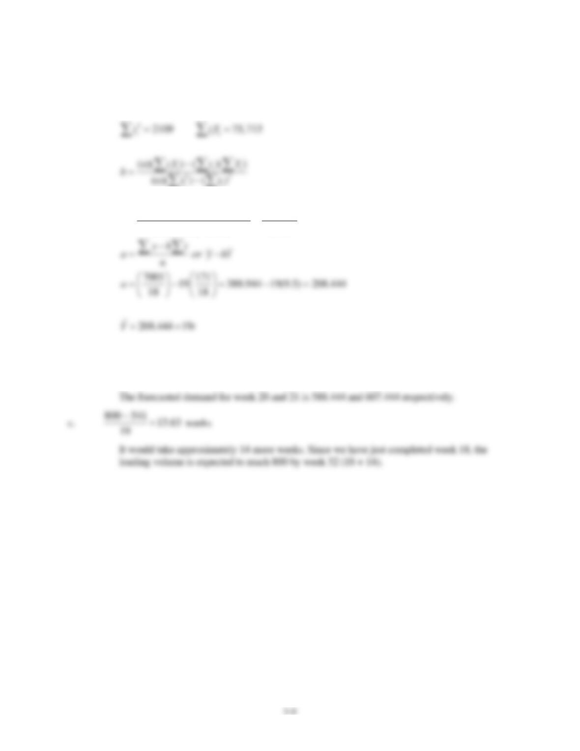
171 7001
(18)(75, 713) (171)(7001) 165, 663 19
(18)(2109) (171) 8721
ii
ii
tY
b
==
−
= = =
−
b. F = 208.444 + (19)(20) = 588.444
F = 208.444 + (19)(21) = 607.444

Chapter 03 – Forecasting
3–10
8.
a.
t
Y
t*Y
t2
1
200
200
1
2
214
428
4
3
211
633
9
4
228
912
16
5
235
1,175
25
6
232
1,332
36
7
248
1,736
49
b = [(15*32136)-(120*3772) / [(15*1240)-1202] = 7.00
a = (3772/15) – [7*(120/15] = 195.47
Y = 195.47 – 7.00t
Forecasted demand for periods 16 through 19 are:
8
250
2,000
64
9
253
2,277
81
281
3,091
275
3,300
280
3,640
288
4,032
310
4,650
3,772
Chapter 03 – Forecasting
3–11
b. Initial Trend =
33.9
3
200228 =
−
Period
Actual
St + Tt = TAFt
TAFt + .3(A – TAFt) = St
Tt–1 + .2 (TAFt – TAFt–1 – Tt–1) = Tt
5
235
228 + 9.33 = 237.33
237.33 + .3(235 – 237.33) = 236.63
9.33
6
232
236.63 + 9.33 = 245.96
245.96 + .3(232 – 245.96) = 241.77
9.33 + .2(245.96 – 237.33 – 9.33) = 9.19
7
248
241.77 + 9.19 = 250.96
250.96 + .3(248 – 250.96) = 250.07
9.19 + .2(250.96 – 245.96 – 9.19) = 8.352
8
250
250.07 + 8.352 = 258.42
258.42 + .3(250 – 258.42) = 255.89
8.352 + .2(258.42 – 250.96 – 8.352) = 8.174
9
253
255.89 + 8.174 = 264.06
264.06 + .3(253 – 264.06) = 260.74
8.174 + .2(264.06 – 258.42 – 8.174) = 7.667
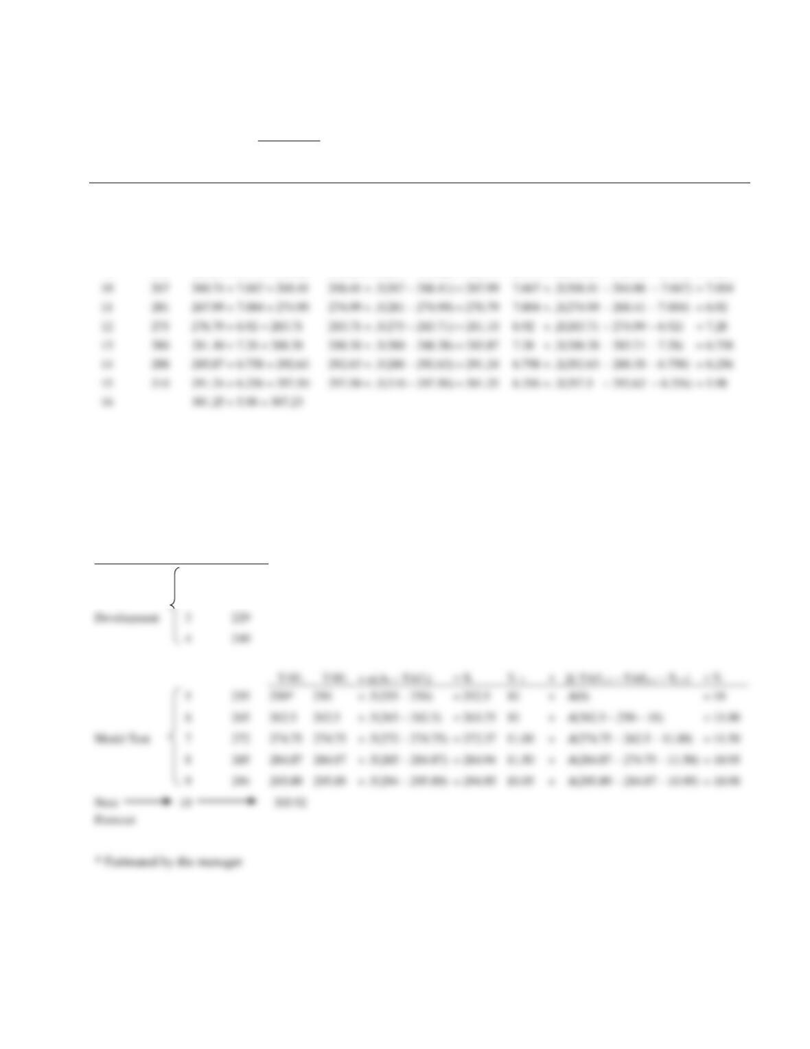
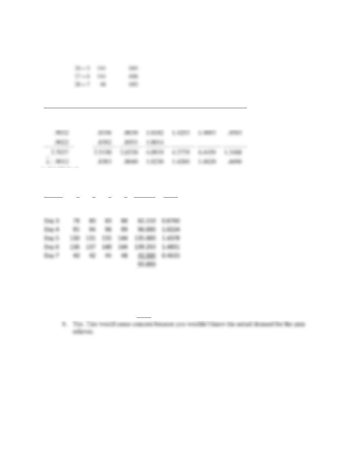
9. The initial estimate of trend is based on the net change of 30 for the three periods from 1 to 4, for
an average of +10 units. Use = .5 and = .4.
Initial trend = (240 – 210)/3 = 10
t Period
At Actual
1
210
Model
2
224
Development
3
229
4
240
5
255
= 252.5
+
.4(0)
= 10
6
265
262.5
262.5
= 263.75
+
= 11.00
Model Test
7
272
274.75
274.75
= 272.37
11.00
+
= 11.50
9
294
295.89
295.89
= 294.95
10.95
+
= 10.98
267
260.74 + 7.667 = 268.41
268.41 + .3(267 – 268.41) = 267.99
7.667 + .2(268.41 – 264.06 – 7.667) = 7.004
281
267.99 + 7.004 = 274.99
274.99 + .3(281 – 274.99) = 276.79
7.004 + .2(274.99 – 268.41 – 7.004) = 6.92
275
276.79 + 6.92 = 283.71
283.71 + .3(275 – 283.71) = 281.10
6.92 + .2(283.71 – 274.99 – 6.92) = 7.28
280
281.10 + 7.28 = 288.38
288.38 + .3(280 – 288.38) = 285.87
7.28 + .2(288.38 – 283.71 – 7.28) = 6.758
285.87 + 6.758 = 292.63
292.63 + .3(288 – 292.63) = 291.24
6.758 + .2(292.63 – 288.38 – 6.758) = 6.256
310
291.24 + 6.256 = 297.50
297.50 + .3(310 – 297.50) = 301.25
6.256 + .2(297.5 – 292.63 – 6.256) = 5.98
301.25 + 5.98 = 307.23

Chapter 03 – Forecasting
3–12
10. Yt = 70 + 5t t = 0 (June of last year)
t = 1 (July of last year)
t = 7 (January of this year)
YJan = 70 + (5)(19) = 165
Forecast = (Trend) * (Seasonal Relative)
Month
Trend * Seasonal Relative
Forecast (Trend * Seasonal Rel)
January
165 * 1.10
181.5
11.
Quarter
I
II
III
IV
I
Value of t
8
9
10
11
12
Trend component, Ft
Quarter relative
1.1
1.0
0.6
1.3
Forecast
Chapter 03 – Forecasting
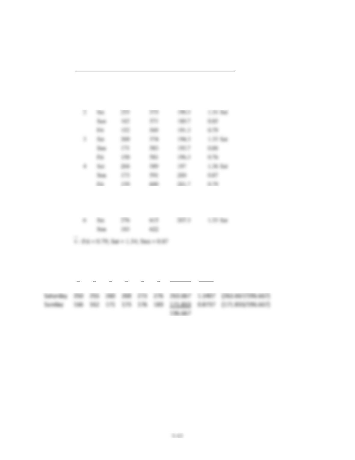
12. . a. Centered Moving Average Method
Week
Day
Sales
Moving
Total
Centered
Moving Av.
Sales/MA5
Fri
149
1
Sat
250
188.3
1.33
Sat
Sun
166
565
190
0.87
Fri
154
570
191.7
0.80
Sun
162
571
189.7
0.85
Fri
152
569
191.3
0.79
Sun
171
583
193.7
0.88
Fri
150
581
196.3
0.76
Sun
173
591
200
0.87
Fri
159
600
201.7
0.79
5
Sat
273
605
202.7
1.35
Sat
Sun
176
608
204
0.86
Fri
163
612
205
0.80
6
Sat
276
615
207.3
1.33
Sat
b. SA Method
WEEK
Season
SA
Season
1
2
3
4
5
6
Average
Index
Friday
149
154
152
150
159
163
154.500
0.7856
(154.500/196.667)
Saturday
250
255
260
268
273
276
263.667
1.3407
(263.667/196.667)
Sunday
166
162
171
173
176
183
171.833
0.8737
(171.833/196.667)
196.667
Overall
Average
c. In this problem, the two methods provide similar results because there are only 3 seasons;
therefore, the two methods are essentially averaging the same data. In addition, there is no trend in the
data.
Chapter 03 – Forecasting
3–14
13. Wednesday = .15 x 4 = 0.60
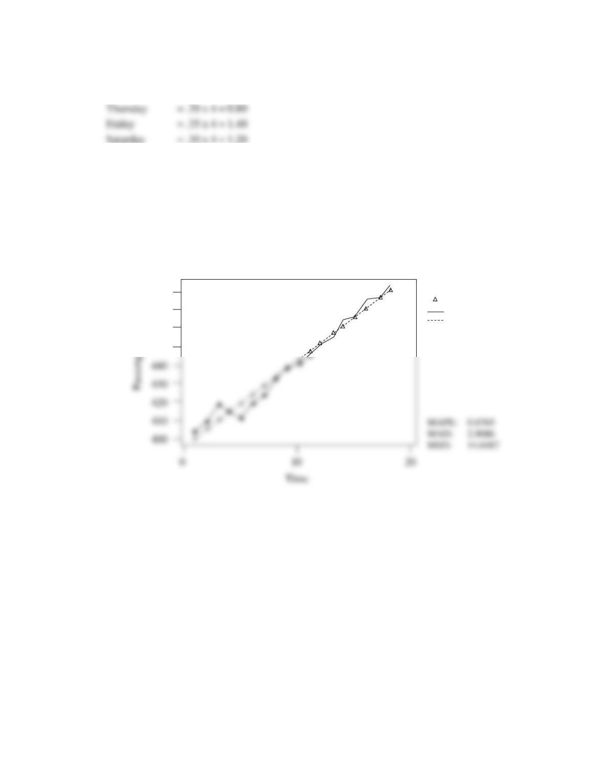
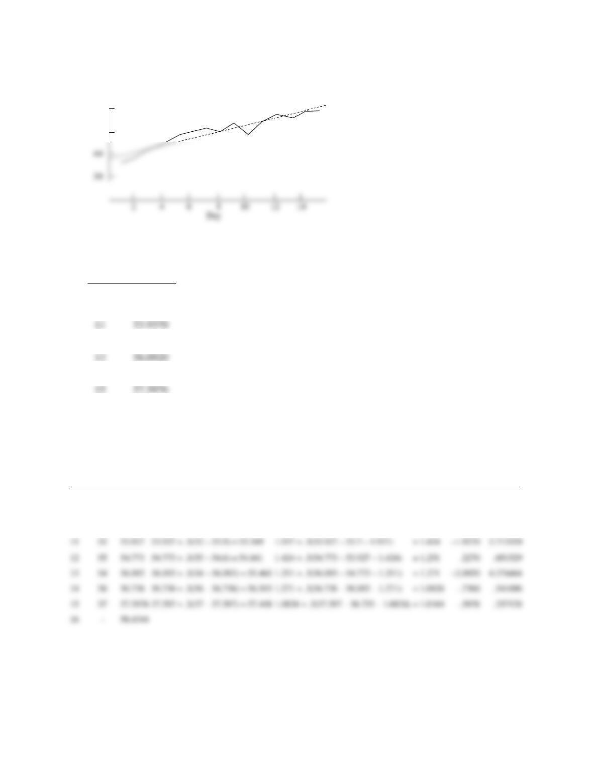
14. a. There appears to be a long-term upward increasing trend in the data. The forecast will
underestimate when data values increase.
b.
•
•
•
•
•
•
•
•
•
480
470
460
450
Actual
Fits
Actual
Fits
Trend Analysis for Passengers
Linear Trend Model
Yt = 396.974 + 4.59340*t
•
•
•
•
•
•
•
•

Chapter 03 – Forecasting
3–15
T
Y
t*Y
t2
1
405
405
1
2
410
820
4
3
420
1260
9
4
415
1660
16
9
438
3942
81
10
440
4400
100
11
446
4906
121
12
451
5412
144
13
455
5915
169
14
464
6496
196
15
466
6990
225
16
474
7584
256
17
476
8092
289
18
482
8676
324
412
2060
25
6
420
2520
36
7
424
2968
49
433
3464
64
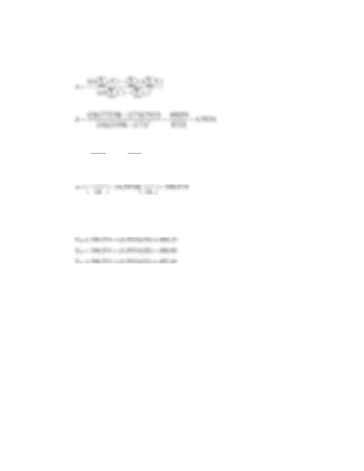
Chapter 03 – Forecasting
3–16
=171
1
t
7931=
i
Y
=77570
iiYt
=2109
2
1
t
tY
n
t
b
n
Y
a
ii
5934.4974.396
)(
+=
−
=
Forecasted demand for the next three weeks are:
Chapter 03 – Forecasting
3–17
15. a. Centered Moving Average Method
Day
(Data)
No. Served
Moving
Total
Centered
Average
(Relative estimates)
Data Centered Average
1 = 1
80
2 = 2
75
3 = 3
78
4 = 4
95
90.57
95/90.57 = 1.0489
5 = 5
130
90.86
130/90.86 = 1.4308
136/91.14 =
10 = 3
80
640
91.57
80/91.57 = .8736
11 = 4
94
639
91.86
94/91.86 = 1.0233
12 = 5
131
640
92.14
125/91.14 = 1.4217
13 = 6
137
641
92.29
135/92.29 = 1.4845
14 = 7
42
643
92.71
42/92.71 = .4530
15 = 1
84
645
93.00
84/93.00 = .9032
16 = 2
78
646
93.57
77/93.57 = .8336
17 = 3
83
649
94.00
83/94.00 = .8830
18 = 4
96
651
94.29
96/94.29 = 1.0182
19 = 5
135
655
94.71
135/94.71 = 1.4253
20 = 6
140
658
95.29
140/95.29 = 1.4693
21 = 7
44
660
96.00
37/96.00 = .4583
22 = 1
87
663
96.43
87/96.43 = .9022
23 = 2
82
667
97.71
82/97.71 = .8392
24 = 3
88
672
98.29
98/98.29 = .8953
25 = 4
99
675
98.86
103/98.86 = 1.0014
6 = 6
136
91.14
7 = 7
40
634
91.43
8 = 1
82
636
91.29
82/91.29 = .8983
9 = 2
77
638
91.43
77/91.43 = .8422
Chapter 03 – Forecasting
3–18
Group and average the relative estimates:
1’s
2’s
3’s
4’s
5’s
6’s
7’s
1.0489
1.4301
1.4922
.4375
.8983
.8422
.8736
1.0233
1.4217
1.4845
.4530
.9032
.8336
.8830
1.0182
1.4253
1.4693
.4583
.9022
.8392
.8953
1.0014
2.5150
2.6520
4.0919
4.2779
4.4459
1.3488
.8383
.8840
1.0230
1.4260
1.4820
.4496
b. SA Method
WEEK
Season
SA
Season
1
2
3
4
Average
Index
Day 1
80
82
84
87
83.250
0.8866
Day 2
75
77
78
82
78.000
0.8307
Day 3
78
80
83
88
82.250
0.8760
Day 4
95
94
96
99
96.000
1.0224
Day 5
130
131
135
144
135.000
1.4378
Day 6
136
137
140
144
139.250
1.4831
Day 7
40
42
44
48
43.500
0.4633
93.893
Overall
Average
16. a. The trend may be non-linear (although most students will view it as linear). Trend-adjusted
smoothing would have a slight edge over a linear trend line.
Chapter 03 – Forecasting
3–19
c.
TAF
9
51.7
10
53.7
12
54.7730
13
56.0920
14
56.7360
16
58.4344
MSE=
6.088
Day
Demand
TAFt
TAFt + .3(At – TAFt) = St
Tt–1 + .3(TAFt – TAFt–1 – Tt–1)
= Tt
ei
2
i
e
8
49
50
50 + .3(49 – 50) = 49.7
2 + .3(50 – 50 – 0 )
= 2
–1
1
9
52
51.7
51.7 + .3(52 – 51.7) = 51.79
2 + .3(51.7 – 50 – 2 )
= 1.91
.3
.09
10
48
53.7
53.7 + .3(48 – 53.7) = 51.99
1.91 + .3(53.7 – 51.7 – 1.91)
= 1.937
–5.7
32.49
11
52
53.927
53.927 + .3(52 – 53.9) = 53.349
1.937 + .3(53.927 – 53.7 – 1.937)
= 1.424
3.713329
13
54
56.092
56.093 + .3(54 – 56.093) = 55.465
1.251 + .3(56.093 – 54.773 – 1.251)
= 1.271
–2.0920
14
56
56.736
56.736 + .3(56 – 56.736) = 56.515
1.271 + .3(56.736 – 56.093 – 1.271)
= 1.0826
15
57
57.5976
57.597 + .3(57 – 57.597) = 57.418
1.0826 + .3(57.597 – 56.735 – 1.0826)
= 1.0164
.357126
16
60
50
Sales
Day
Chapter 03 – Forecasting
3–20
17.
Month
Units
Sold
Index
Month
Units
Sold
Index
Jan……….
640
0.80
Jul. ……….
765
0.90
Feb. ……..
648
0.80
Aug. ……..
805
1.15
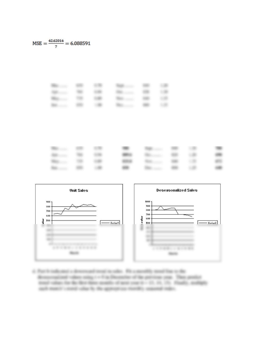
Solution
Month
Units
Sold
Index
Deseasonalized
Month
Units
Sold
Index
Deseasonalized
Jan……….
640
0.80
800
Jul. ………..
765
0.90
850
Feb. ……..
648
0.80
810
Aug. ………
805
1.15
700
Mar. …….
630
0.70
900
Sept. ……..
840
1.20
700
Apr. ……..
761
0.94
Oct. ……….
828
1.20
690
May ……..
735
0.89
Nov. ………
840
1.25
672
Jun. ……..
850
1.00
850
Dec. ………
800
1.25
640
e. Advertising and sales promotions.
Mar. …….
630
0.70
Sept. ……..
840
1.20
Apr. ……..
761
0.94
Oct. ………
828
1.20
May ……..
735
0.89
Nov. ……..
840
1.25
Jun. ……..
850
1.00
Dec. ………
800
1.25