EXERCISE 3-4 3-21
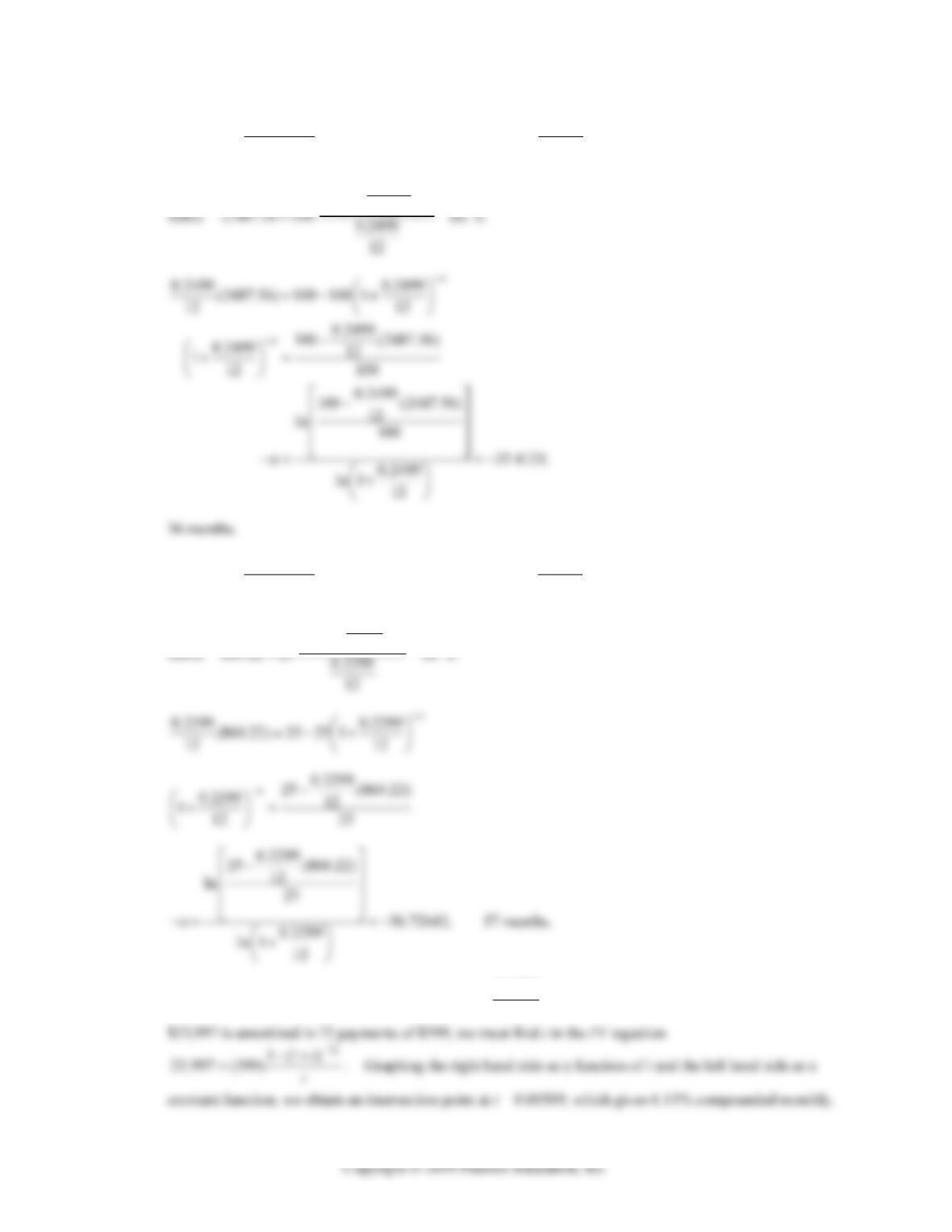
34. 1 (1 ) 0.2499
; 2,487.56, 100, .
12
n
i
PV PMT PV PMT i
i
0.2499
11 12
n
36. 1 (1 ) 0.2299
; 860.22, 25.00, .
12
n
i
PV PMT PV PMT i
i
0.229
11 12
n
0.2299
ln 1 12
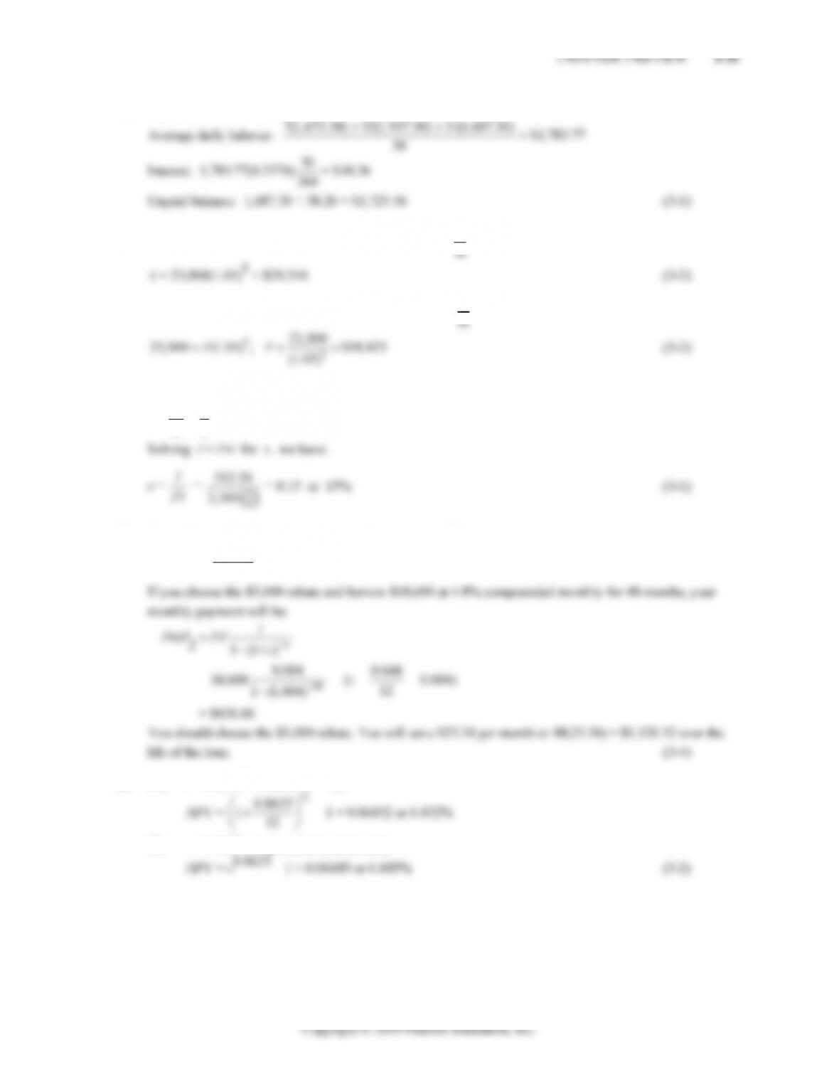
38. For 0% financing, the monthly payments should be 23,997 333.29
72 = $333.29, not $399. If a loan of
EXERCISE 3-4 3-23
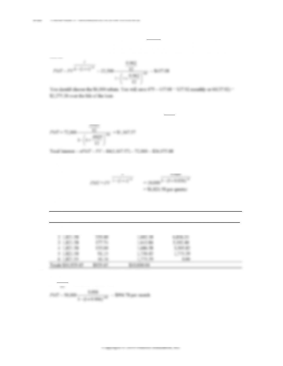
The amount, D, in the account at the end of first year is the present value of a 4 year annuity:
48
1(10.006)
= $41,381.67
48. Amortized amount = 120,000 – (120,000)(0.20) = $96,000.
Thus PV = $96,000, n = 12(30) = 360, r = 7.5% = 0.075,
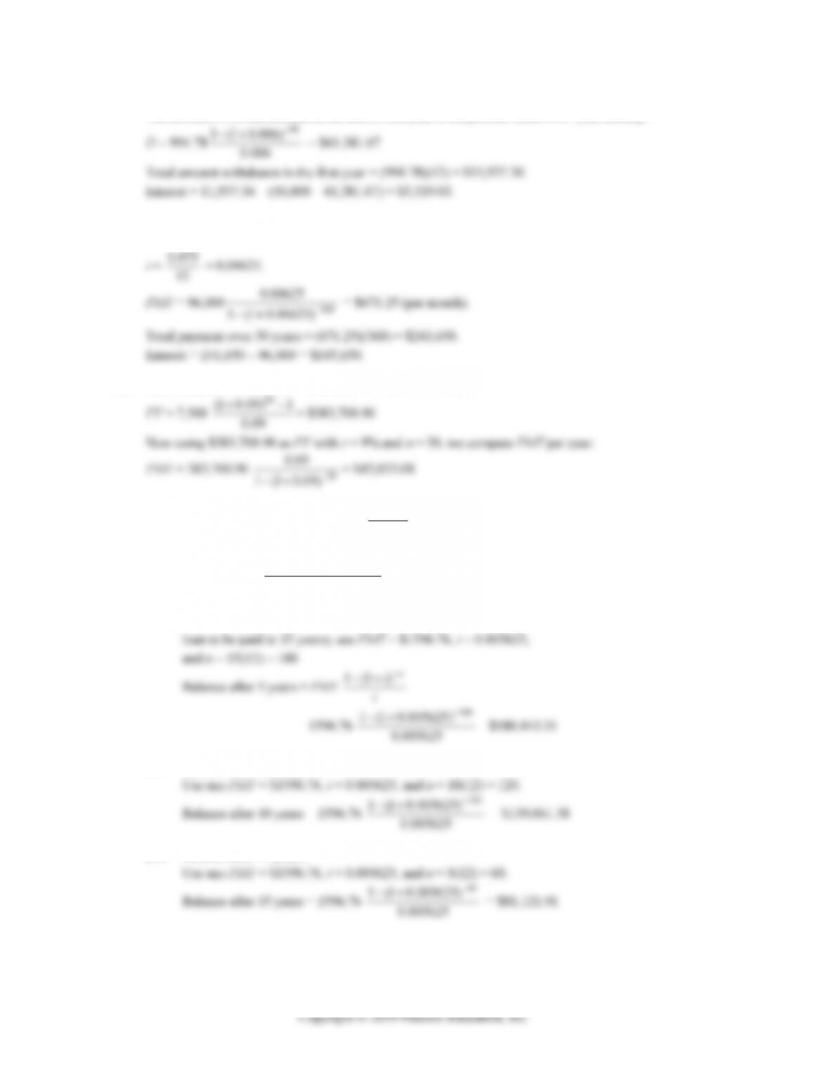
50. First, compute FV for PMT = $7,500, r = 9% = 0.09, n = 20:
20
(1 0.09) 1
52. PV = $210,000, r = 6.75% = 0.0675, i = 0.0675
12 = 0.005625;
n = 240.
Thus PMT = 210,000 240
0.005625
1 (1 0.005625)
= $1596.76 (per month)
(A) Now to compute the balance after 5 years (with balance of the
= 1596.76
0.005625
(B) Balance after 10 years:
Balance after 10 years = 1596.76
0.005625
(C) Balance after 15 years:
Balance after 15 years = 1596.76
0.005625
3-24 CHAPTER 3: MATHEMATICS OF FINANCE
54. (A) PV = $200,000, r = 8.4% = 0.084, m = 12, i = 0.084
12 = 0.007,
(B) PMT = $3,000, r = 8.4% = 0.084, i = 0.007, PV = $200,000
n
56. Using the information in Problem 55, the balance B in the account after k years is:
12 12
kk
58. (A) First, calculate the present value of the ordinary annuity:
PMT = $1,500, i = 0.0648
EXERCISE 3-4 3-25
(B) First, calculate the FV with PMT = $1,000, i = 0.0054,
n = 15(12) = 180
180
(1.0054) 1
= $303,022.71
60. Amortized amount = $160,000 – (160,000)(0.20) = $128,000.
Thus, PV = $128,000, i = 0.00646, n = 360.
PMT = 128,000 360
0.00646
62. PV = $200,000 – (0.20)(200,000) = $160,000
D = 1,794.97
1(10.011)
.011
= $119,272.89
PMT = 119,272.89 120
0.082
12
= $1,459.74
64. All three graphs are decreasing, curve downward, and have the same x and y intercepts; the greater the
CHAPTER 3 REVIEW 3-27
CHAPTER 3 REVIEW
1. A = 100 0.09
12
2. 808 = P0.12
112
3. 212 = 200(1 + 0.08·t) 4. 4,120 = 4,000 1
1·
2
r
r= 4,120
(3-1)
5. A = 1,200(1 + 0.005)30
(3-2)
6. P = 60
5, 000
n
A
5,000
(3-2)
7. A = Pert; P = 4,750, r = 6.8% = 0.068, t = 3
8. A = Pert; A = 36,000, r = 9.3% = 0.093, t = 60 months = 5 years
36,000
= $69,770.03 (3-3)
11.
16
1(10.02)
2,500 0.02
PV
12. 60
(0.0075)8,000
1 (1 0.0075)
PMT
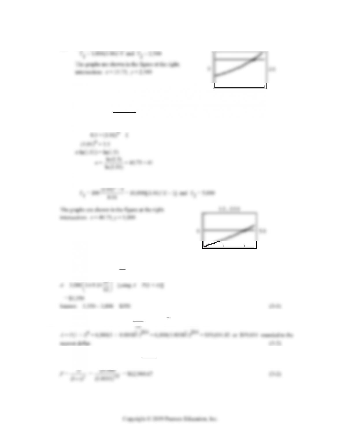
13. (A) 2,500 = 1,000(1.06)n
(1.06)n = 2.5
3-28 CHAPTER 3: MATHEMATICS OF FINANCE
(B) We find the intersection of
3000
0 (3-2)
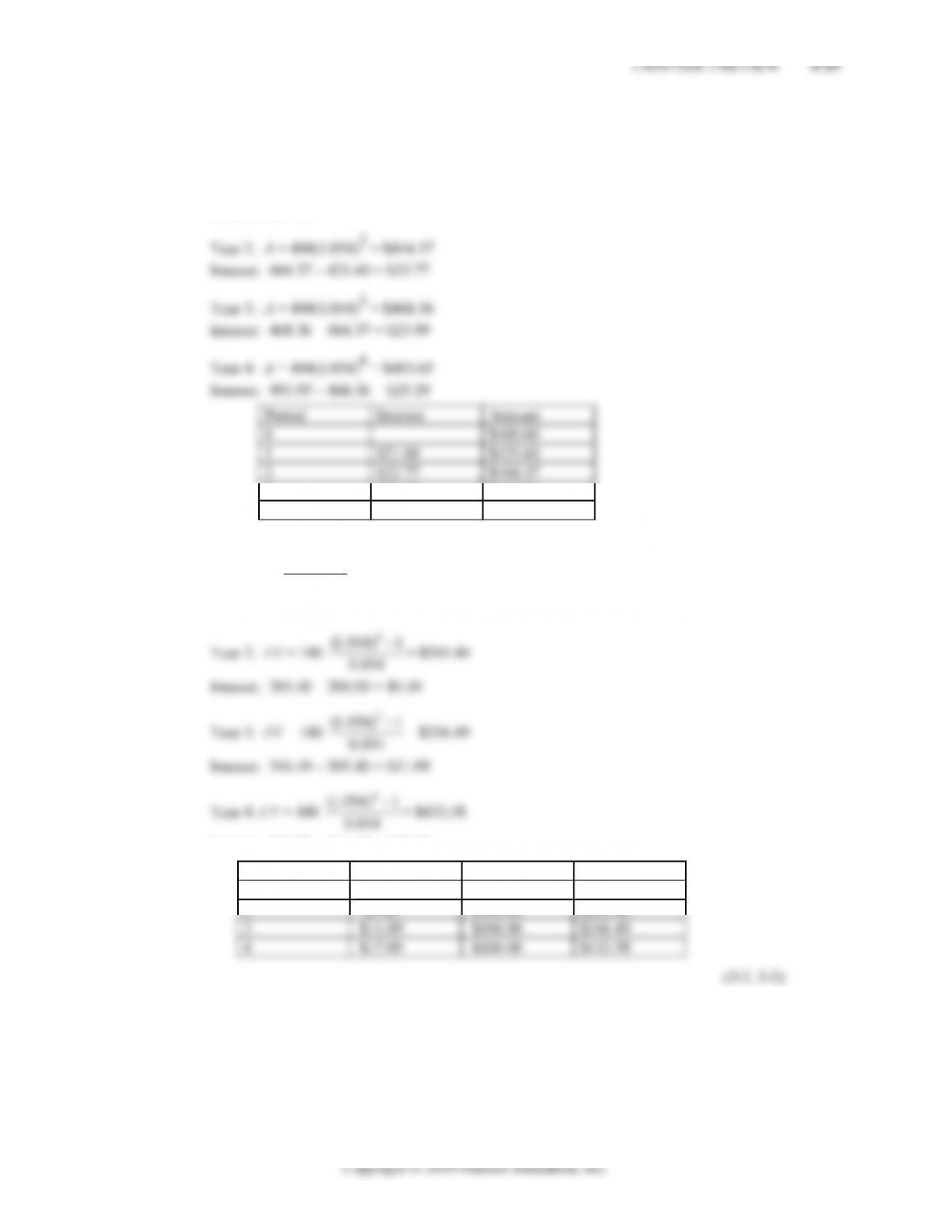
14. (A) 5,000 = 100 (1.01) 1
0.01
n
5,000 = 10,000[(1.01)n – 1]
(B) We find the intersection of
x= 10,000[(1.01)^X – 1] and Y2 = 5,000
intersection: x = 40.75; y = 5,000
050
0 (3-3)
15. P = $3,000, r = 0.14, t = 10
12
16. P = $6,000, r = 7% = 0.07, i = 0.07
0.00583
, n = 17(12) = 204
17. A = $25,000, r = 6.6% = 0.066, i = 0.066
12 = 0.0055, n = 10(12) = 120
A
25,000
3-30 CHAPTER 3: MATHEMATICS OF FINANCE
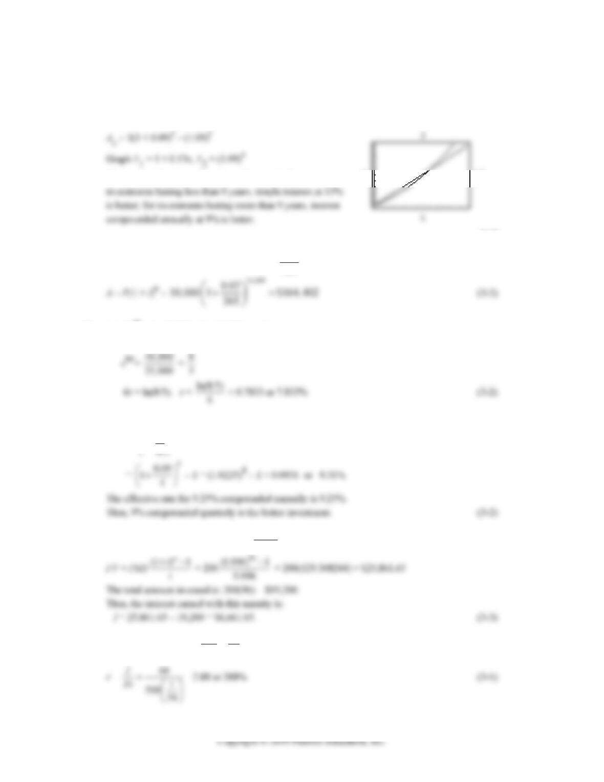
19. The value of $1 at 13% simple interest after t years is:
As = 1(1 + 0.13t) = 1 + 0.13t
The value of $1 at 9% interest compounded annually for t years is:
The graphs intersect at the point where x ≈ 9. For
3
0 15
(3-2)
20. P = $10,000, r = 7% = 0.07, m = 365, i = 0.07
365 , and n = 40(365) = 14,600
14,600
0.07
21. A = Pert; A = 40,000, P = 25,000, t = 6
40,000 = 25,000e6r
22. The effective rate for 9% compounded quarterly is:
APY = 1
m
r
– 1, r = 0.09, m = 4
4
0.09
23. PMT = $200, r = 7.2% = 0.072, i = 0.072
12 = 0.006, n = 8(12) = 96
n
i
96
(1.006) 1
= 200(129.308244) = $25,861.65
24. P = $500, I = $60, t = 15 1
360 24
year.
1
500 24
I
Pt