Chapter 03 – Forecasting
3–21
18. Deseasonalize the values, where:
Deseasonalized sales = (Actual sales) / (Seasonal relative)
Deseasonalized sales for quarter 1 is (88) / (1.1) = 80
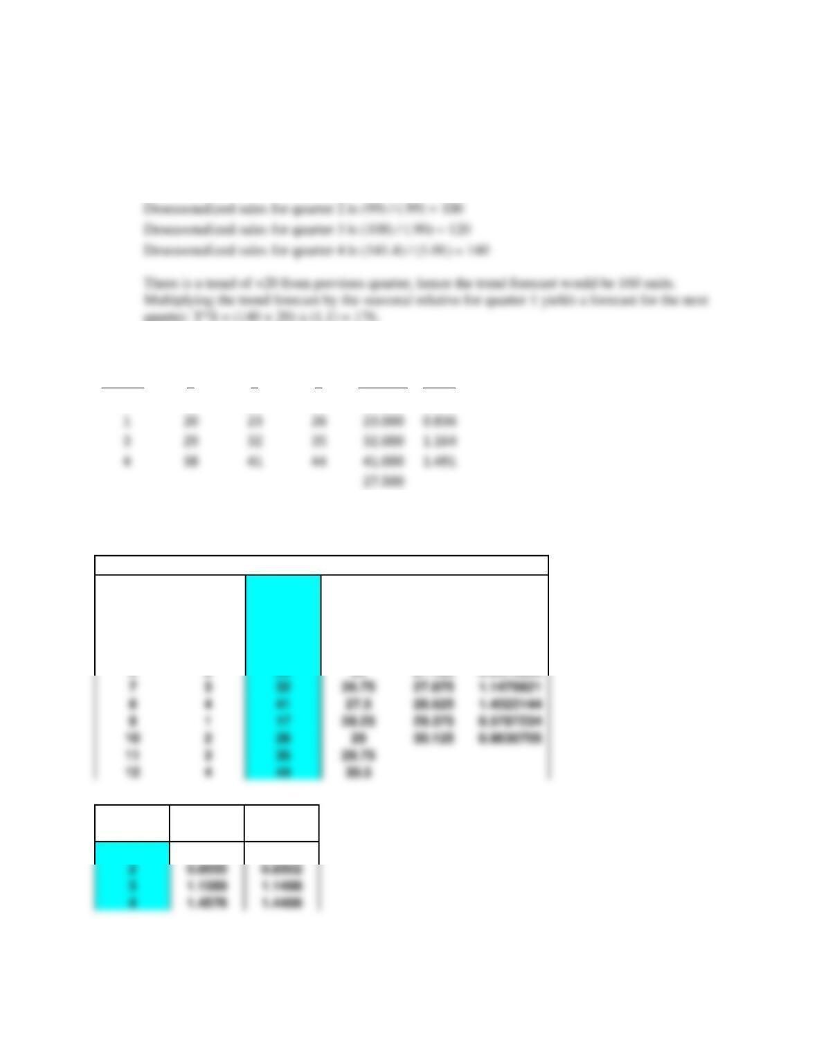
19. a. SA Method
WEEK
Season
SA
Season
1
2
3
Average
Index
1
11
14
17
14.000
0.509
1
20
23
26
23.000
0.836
3
29
32
35
32.000
1.164
4
38
41
44
41.000
1.491
27.500
Overall
Average
b. Centered Moving Average Method
Period
Season
Actual
MA
Center
Index
1
1
11
#N/A
#N/A
2
2
20
#N/A
#N/A
3
3
29
#N/A
24.875
1.1658291
4
4
38
24.5
25.625
1.4829268
5
1
14
25.25
26.375
0.5308057
6
2
23
26
27.125
0.8479263
7
3
32
26.75
27.875
1.1479821
8
4
27.5
28.625
1.4323144
9
1
17
28.25
29.375
0.5787234
10
2
26
29
30.125
0.8630705
11
3
35
29.75
#N/A
12
4
44
30.5
#N/A
Season
Average
Standard
Index
Index
1
0.5548
0.5513
2
0.8555
0.8502
3
1.1569
1.1498
4
1.4576
1.4486
c. The Centered Moving Average method is better because there is a trend in the data.
Chapter 03 – Forecasting
3–22
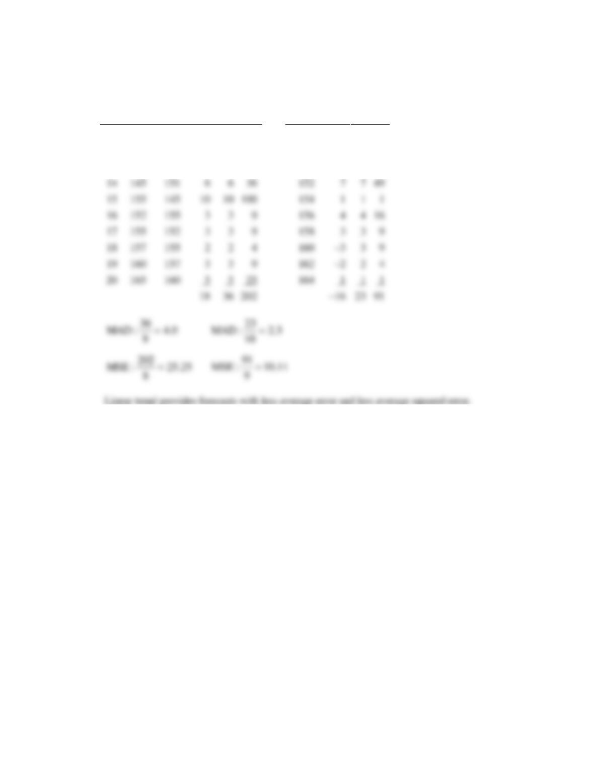
20.
t
Units
sold
Naive
e
| e |
e2
Trend
e
| e |
e2
11
147
−
146
1
1
1
12
148
147
1
1
1
148
0
0
0
13
151
148
3
3
9
150
1
1
1
14
145
151
6
152
7
15
155
145
154
1
1
1
16
152
155
3
9
156
4
18
157
155
2
2
4
160
3
9
19
160
157
3
3
9
162
2
4
20
165
160
164

Chapter 03 – Forecasting
3–23
21.
Period
Demand
F1
e
e
e2
F2
e
e
e2
1
68
66
2
2
4
66
2
2
4
2
75
68
7
7
49
68
7
7
49
3
70
72
–2
2
4
70
0
0
0
32
176
24
106
a. MAD F1: 32/8 = 4.0
MAD F2: 24/8 = 3.0 F2 appears to be more accurate.
b. MSE F1: 176/7 = 25.14
MSE F2: 106/7 = 15.14 F2 appears to be more accurate.
22.
a.
Forecast #1
Forecast #2
Month
A
Sales
F Forecast
(A–F)
Error
Error2
| e |
Forecast
Error
Error2
| e |
1
770
771
–1
1
1
769
1
1
1
2
789
785
4
16
4
787
2
4
2
3
794
790
4
16
4
792
2
4
2
4
780
784
–4
16
4
798
–18
324
18
5
768
770
–2
4
2
774
36
6
6
772
768
4
16
4
770
2
4
2
7
760
761
–1
1
1
759
1
1
1
9
786
784
2
4
2
788
4
2
790
788
2
2
788
4
2
12
94
28
–16
382
36
4
74
71
3
9
72
2
4
5
69
72
–3
3
9
74
5
25
6
72
70
2
4
76
4
16
7
80
71
9
9
81
78
2
2
4
8
78
74
4
16
80
4
Chapter 03 – Forecasting
3–24
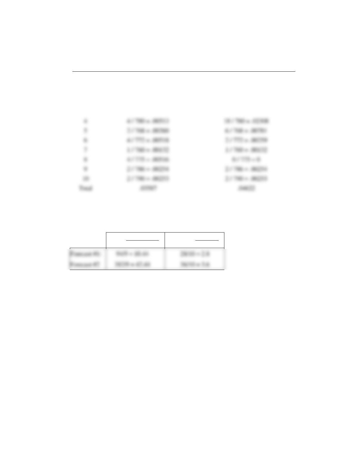
b.
Period
Absolute Percentage Error (F1)
Absolute Percentage Error (F2)
1
1 / 770 = .00130
1 / 770 = .0013
2
4 / 789 = .00507
2 / 789 = .00253
3
4 / 794 = .00504
2 / 794 = .00252
MAPE F1 = .03587 / 10 = .003587
MAPE F2 = .04622 /10 = .004622
Since .003587 < .004622, choose forecasting method 1.
MSE =
(A – F) 2
MAD =
| e |
n – 1
N
4
4 / 780 = .00513
6
4 / 772 = .00518
2 / 772 = .00259
7
1 / 760 = .00132
1 / 760 = .00132
9
2 / 786 = .00254
2 / 786 = .00254
2 / 790 = .00253
2 / 790 = .00253
Chapter 03 – Forecasting
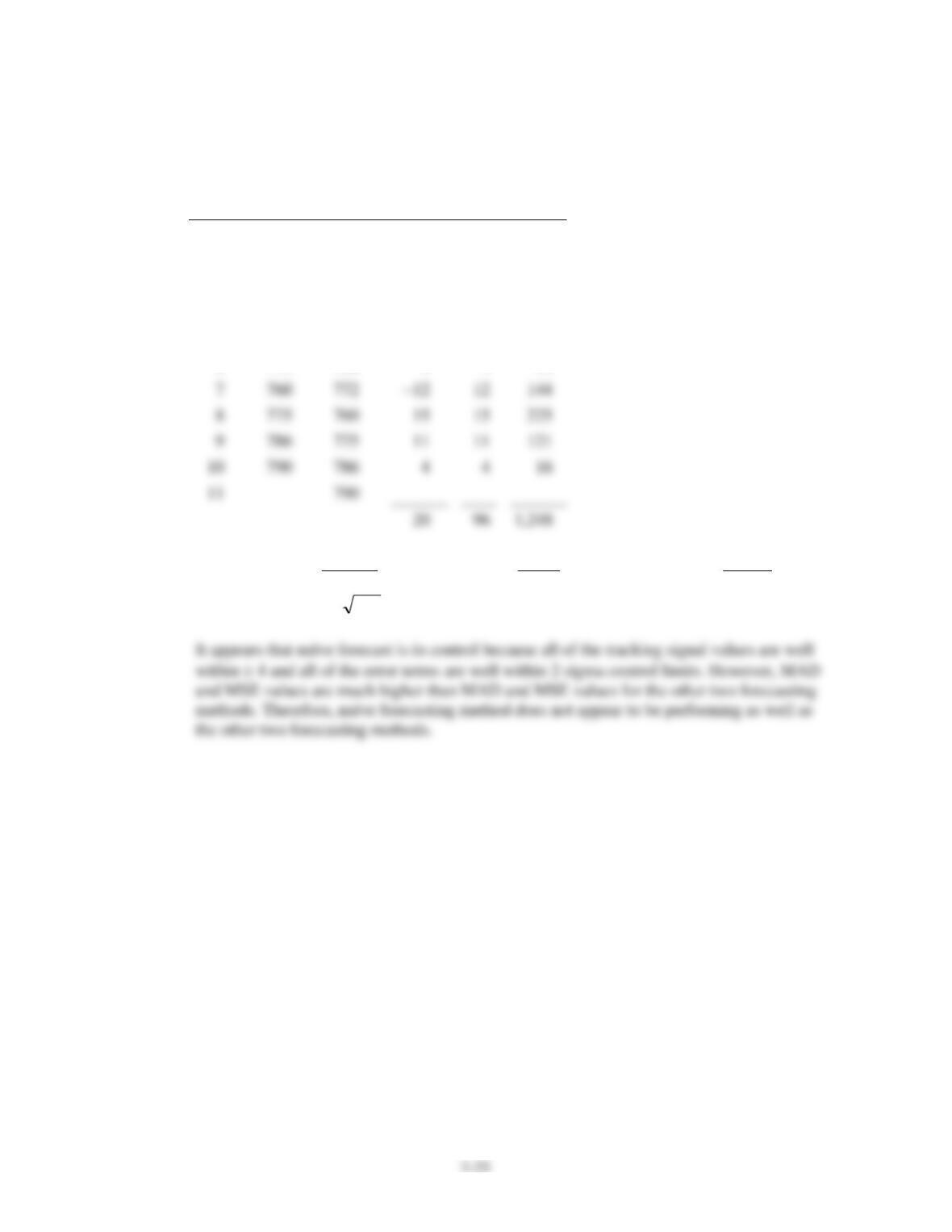
c.
Month
Sales
Naïve
Forecast
(A – F)
Error
| e |
Error2
1
770
2
789
770
19
19
361
3
794
789
5
5
25
4
780
794
–14
14
196
5
768
780
–12
12
144
6
772
768
4
4
16
7
760
772
8
775
760
15
15
225
9
786
775
11
11
121
10
790
786
4
4
16
11
790
MSE =
1,248
= 156
MAD =
96
= 10.67
Tracking
Signal
=
20
= 1.87
8
9
10.67
Control limits: 0 2
156
= 0 25 [in control]
Chapter 03 – Forecasting
3–26
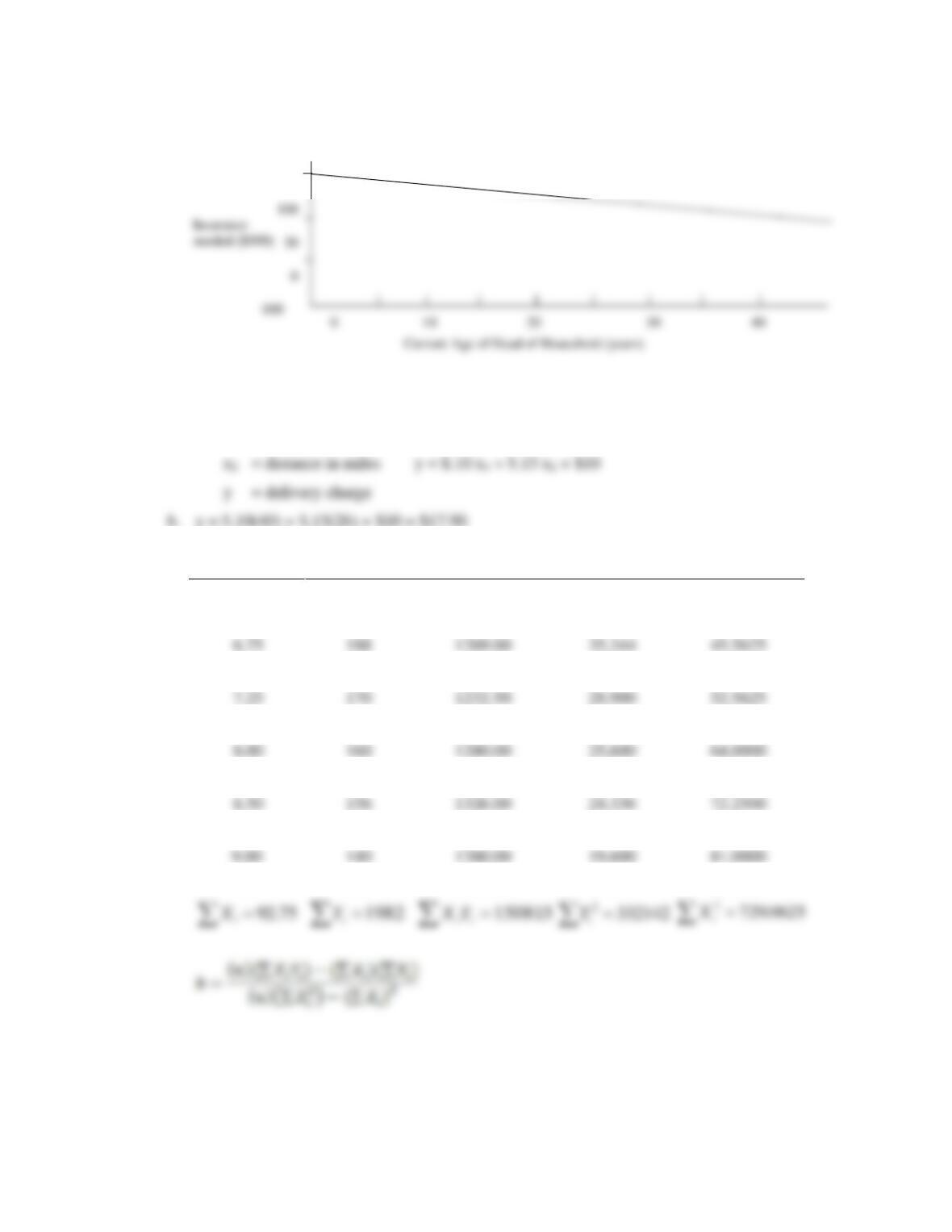
23. a.
b. y = 150 – .1(30) = 147. Thus, a 30-year old will need $147,000 of life insurance.
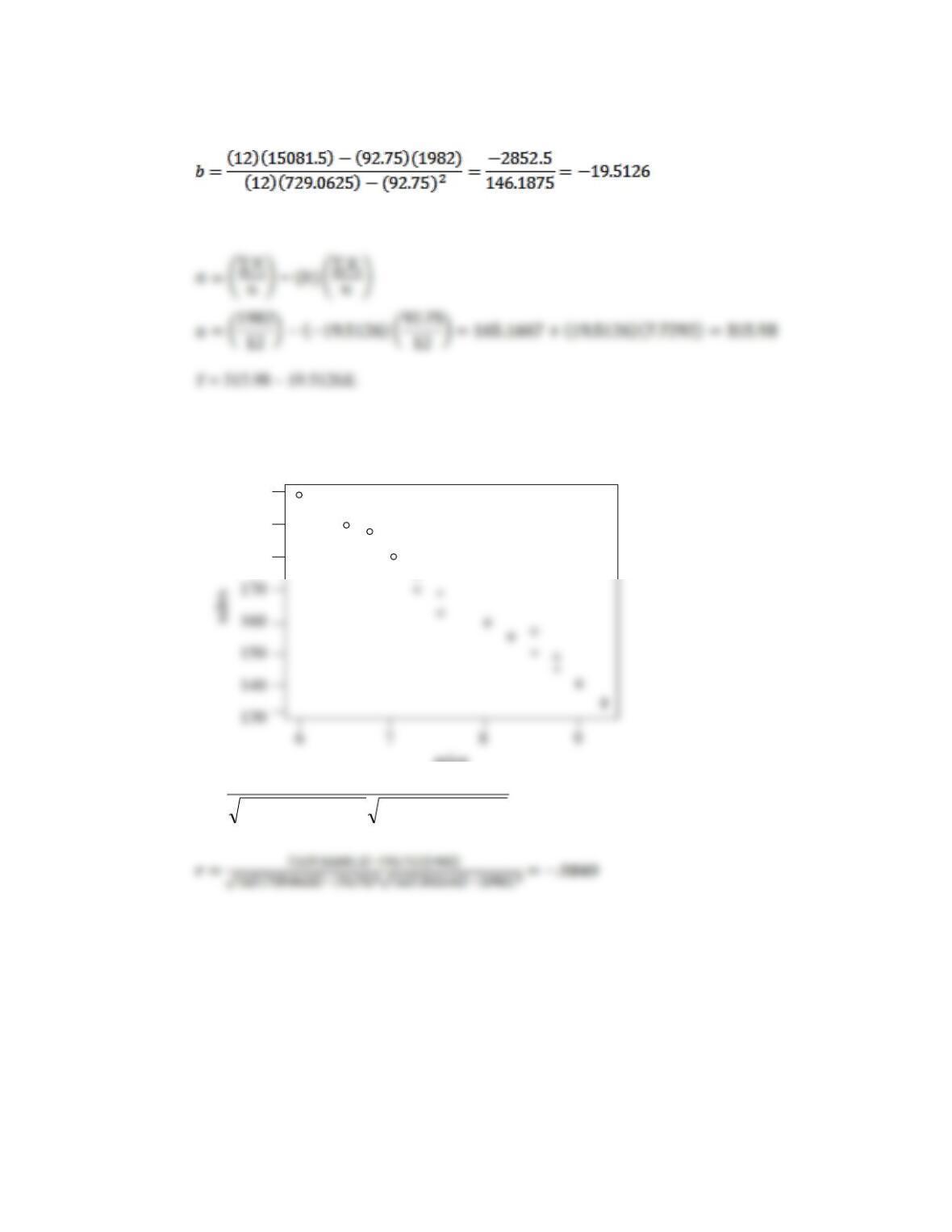
24. a. Let x1 = weight in lb.
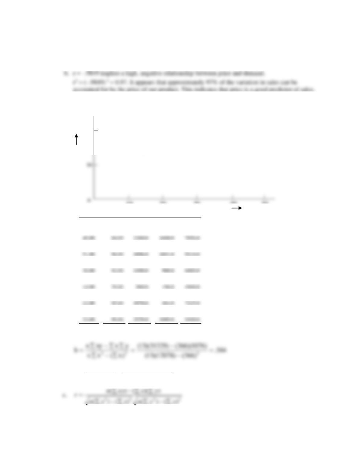
25. a.
X = Price
Y = Sales
X*Y
Y2
X2
6.00
200
1200.00
40,000
36.0000
6.50
190
1235.00
36,100
42.2500
6.75
188
1269.00
35,344
45.5625
7.00
180
1260.00
32,400
49.0000
7.25
170
1232.50
28,900
52.5625
7.50
162
1215.00
26,244
56.2500
8.00
160
1280.00
25,600
64.0000
8.25
155
1278.75
24,025
68.0625
8.50
156
1326.00
24,336
72.2500
8.75
148
1295.00
21,904
76.5625
9.00
140
1260.00
19,600
81.0000
9.25
133
1230.25
17,689
85.5625
150
Chapter 03 – Forecasting
3–27
Actual data are represented by circles.
Predicted values are represented by pluses.
+
+
+
+
2222 )()()()(
))(()(
yynxxn
yxxyn
r−−
−
=
+
price
200
190
180
+
+
+
+
Chapter 03 – Forecasting
3–28
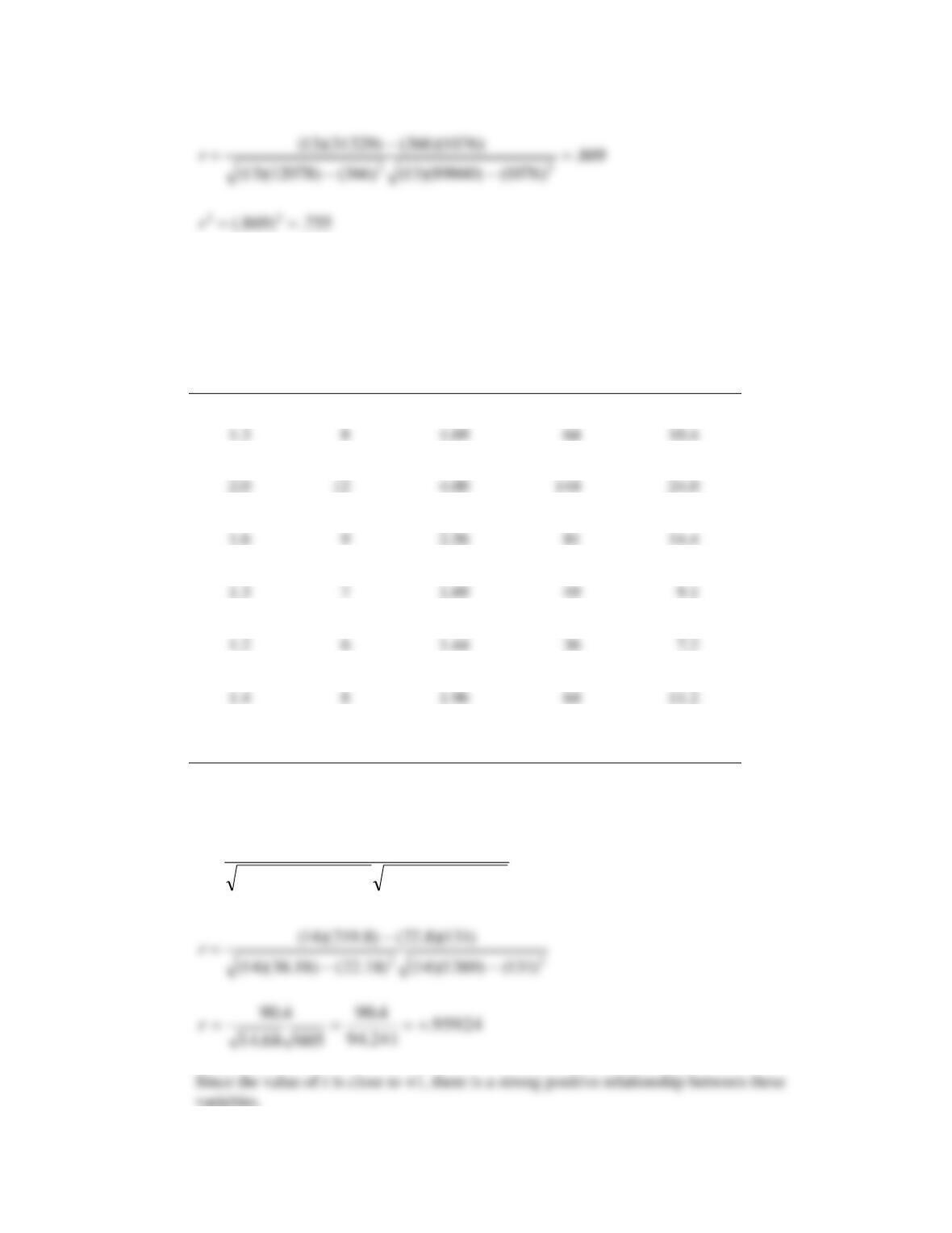
26. a.
b.
x
y
xy
x2
y2
15.00
74.00
1110.0
225.0
5476.0
25.00
80.00
2000.0
625.0
6400.0
32.00
81.00
2592.0
1024.0
6561.0
51.00
96.00
4896.0
2601.0
9216.0
47.00
95.00
4465.0
2209.0
9025.0
30.00
83.00
2490.0
900.0
6889.0
18.00
78.00
1404.0
324.0
6084.0
14.00
70.00
980.0
196.0
4900.0
15.00
72.00
1080.0
225.0
5184.0
22.00
85.00
1870.0
484.0
24.00
88.00
2112.0
576.0
7744.0
33.00
90.00
2970.0
1089.0
8100.0
366.00
1076.00
31329.0
12078.0
89860.0
33.66
13
)366)(584(.1076
n
xby
a
=
−
=
−
=
•
•
•
10 20 30 40 50
y
x
•
•
•
•
•
•
•
•
•
•
100
•
•
•
•
•
•
•
•
•
•
•
•
•
Chapter 03 – Forecasting
3–29
Approximately 75% of the variation in the dependent variable is explained by the
independent variable.
d. y = 66.33 + .584 (41) = 90.268.
27. a. Fertilizer Mower
(X)
(Y)
(X2)
(Y2)
(X)*(Y)
1.6
10
2.56
100
16.0
1.3
8
1.69
64
10.4
1.8
11
3.24
121
19.8
2.0
12
4.00
144
24.0
2.2
12
4.84
144
26.4
1.6
9
2.56
81
14.4
1.5
8
2.25
64
12.0
1.3
7
1.69
49
9.1
1.7
10
2.89
100
17.0
1.2
6
1.44
36
7.2
1.9
11
3.61
121
20.9
1.4
8
1.96
64
11.2
1.7
10
2.89
100
17.0
1.6
9
2.56
81
14.4
22.8
131
38.18
1269
219.8
Answers to parts a and b
2222 )()()()(
))(()(
iiii
iiii
YYnXXn
YXYXn
r−−
−
=
Chapter 03 – Forecasting
3–30
ii
a
n
X
b
n
Y
a
672.)6286.1)(158.6(3571.9
14
8.22
)158.6(
14
131
)(
−=+=
−
=
−
=
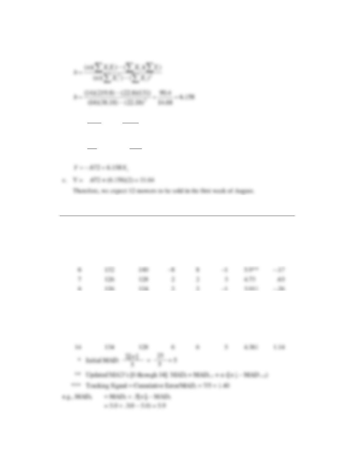
28.
t
Period
A
Demand
F
Predicted
E
Error
| e |
Cum.
Error
MADt
Tracking
Signal
1
129
124
5
5
5
2
194
200
–6
6
–1
3
156
150
6
6
5
4
91
94
–3
3
2
5
85
80
5
5
7
5*
1.40***
6
132
140
–8
8
–1
5.9**
–.17
7
128
–2
2
–3
4.73
–.63
8
126
124
2
2
–1
3.911
–.26
9
95
100
–5
5
–6
4.238
–1.42
10
149
150
–1
1
–7
3.267
–2.14
11
98
94
4
4
–3
3.487
–.86
12
85
80
5
5
2
3.941
.51
13
137
140
–3
3
–1
3.659
–.27
14
134
128
6
6
5
4.361
1.14
Chapter 03 – Forecasting
3–31
Since all tracking signal values are within the limits, the forecast is in control.
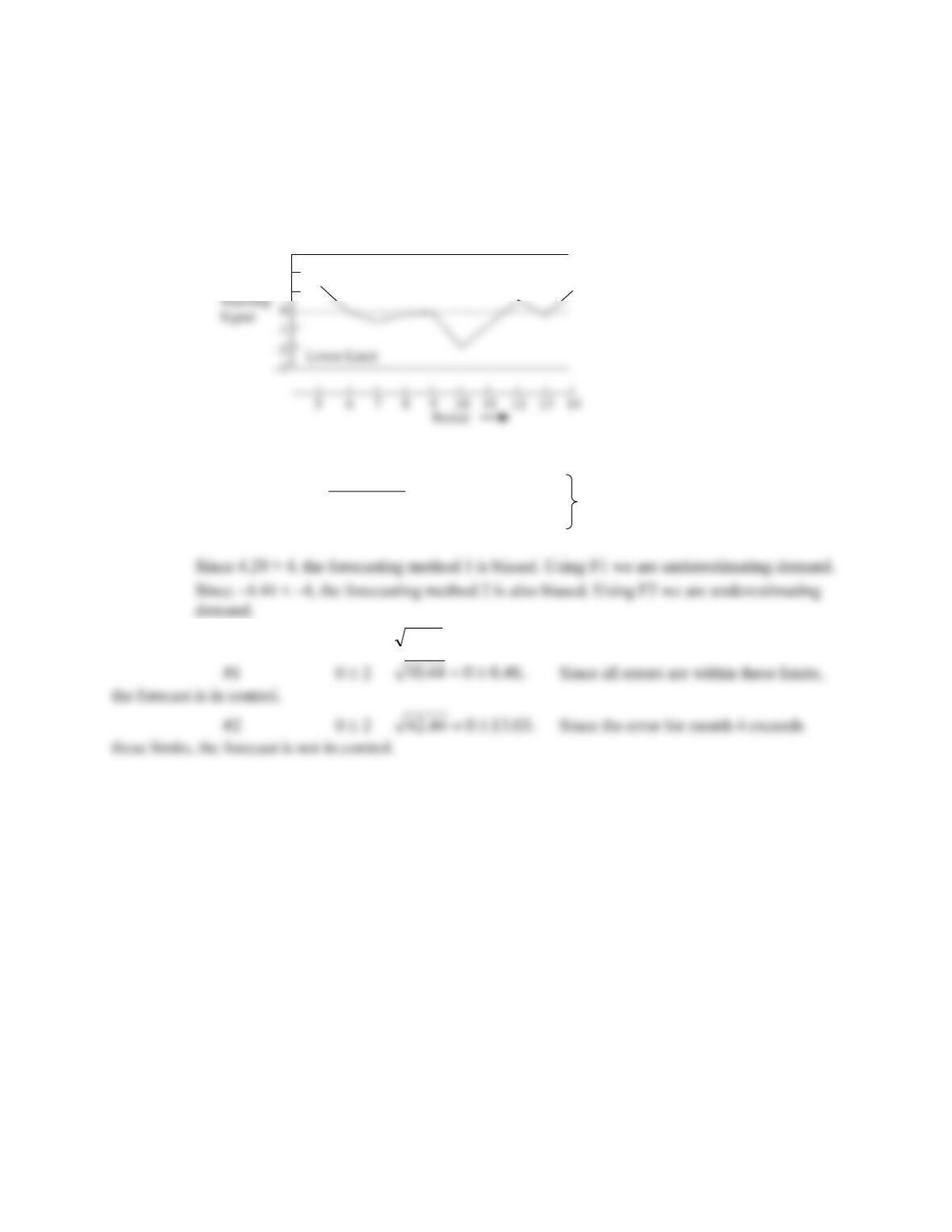
29. Refer to data in problem 22
a.
Tracking signal =
Errors
#1:
12/2.8 =
4.29
[both slightly beyond limits of 4]
MAD
#2:
–16/3.6 =
–4.44
b. Control limits are 0 2
MSE
Value of
Upper Limit
3
2
1
Lower Limit
5 6 7 8 9 10 11 12 13 14
Period
Chapter 03 – Forecasting
3–32
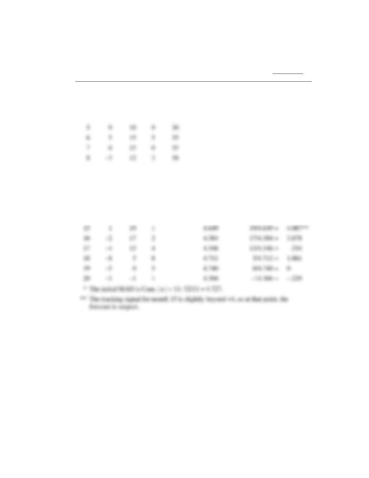
30. a.
MAD t = MAD t–1
+ .1[ | e | t – MAD t–1]
T.S. =
Cum. Error
MAD t
t
Month
e
Error
Cum.
Error
| e |t
Cum.
| e |
1
–8
–8
8
8
2
–2
–10
2
10
3
4
–6
4
14
4
7
1
7
21
9
–9
3
9
47
10
–4
–1
4
51
11
1
0
1
52
4.727*
0/4.727 =
0
12
6
6
6
4.857
6/4.857 =
1.235
13
8
14
8
5.171
14/5.171 =
2.707
14
4
18
4
5.054
18/5.054 =
3.562
15
1
1
4.649
19/4.649 =
4.087**
16
–2
17
2
4.384
17/4.384 =
3.878
17
–4
13
4
4.346
13/4.346 =
18
–8
5
8
4.711
5/4.711 =
1.061
19
0
5
4.740
0/4.740 =
0
20
–1
–1
1
4.366
5
9
10
9
30
6
5
15
5
35
7
0
15
0
35
8
3
38