Tracking Signal
34 #N/A #N/A
35 #N/A #N/A
36 #N/A #N/A
37 #N/A #N/A
48 #N/A #N/A
49 #N/A #N/A
50 #N/A #N/A
51 #N/A #N/A
52 #N/A #N/A
53 #N/A #N/A
54 #N/A #N/A
55 #N/A #N/A
56 #N/A #N/A
57 #N/A #N/A
58 #N/A #N/A
59 #N/A #N/A
60 #N/A #N/A
61 #N/A #N/A
62 #N/A #N/A
63 #N/A #N/A
64 #N/A #N/A
65 #N/A #N/A
66 #N/A #N/A
67 #N/A #N/A
68 #N/A #N/A
69 #N/A #N/A
70 #N/A #N/A
71 #N/A #N/A
72 #N/A #N/A
73 #N/A #N/A
74 #N/A #N/A
Page 61
38 #N/A #N/A
39 #N/A #N/A
40 #N/A #N/A
41 #N/A #N/A
42 #N/A #N/A
43 #N/A #N/A
44 #N/A #N/A
45 #N/A #N/A
46 #N/A #N/A
47 #N/A #N/A
Tracking Signal
75 #N/A #N/A
76 #N/A #N/A
77 #N/A #N/A
78 #N/A #N/A
79 #N/A #N/A
80 #N/A #N/A
91 #N/A #N/A
92 #N/A #N/A
93 #N/A #N/A
94 #N/A #N/A
95 #N/A #N/A
96 #N/A #N/A
97 #N/A #N/A
98 #N/A #N/A
99 #N/A #N/A
100 #N/A #N/A
101 #N/A #N/A
102 #N/A #N/A
103 #N/A #N/A
104 #N/A #N/A
105 #N/A #N/A
106 #N/A #N/A
107 #N/A #N/A
108 #N/A #N/A
109 #N/A #N/A
110 #N/A #N/A
111 #N/A #N/A
112 #N/A #N/A
113 #N/A #N/A
114 #N/A #N/A
115 #N/A #N/A
Page 62
81 #N/A #N/A
82 #N/A #N/A
83 #N/A #N/A
84 #N/A #N/A
85 #N/A #N/A
86 #N/A #N/A
87 #N/A #N/A
88 #N/A #N/A
89 #N/A #N/A
90 #N/A #N/A
Tracking Signal
116 #N/A #N/A
117 #N/A #N/A
118 #N/A #N/A
119 #N/A #N/A
120 #N/A #N/A
121 #N/A #N/A
122 #N/A #N/A
123 #N/A #N/A
134 #N/A #N/A
135 #N/A #N/A
136 #N/A #N/A
137 #N/A #N/A
138 #N/A #N/A
139 #N/A #N/A
140 #N/A #N/A
141 #N/A #N/A
142 #N/A #N/A
143 #N/A #N/A
144 #N/A #N/A
145 #N/A #N/A
146 #N/A #N/A
147 #N/A #N/A
148 #N/A #N/A
149 #N/A #N/A
150 #N/A #N/A
151 #N/A #N/A
152 #N/A #N/A
153 #N/A #N/A
154 #N/A #N/A
155 #N/A #N/A
156 #N/A #N/A
Page 63
124 #N/A #N/A
125 #N/A #N/A
126 #N/A #N/A
127 #N/A #N/A
128 #N/A #N/A
129 #N/A #N/A
130 #N/A #N/A
131 #N/A #N/A
132 #N/A #N/A
133 #N/A #N/A
Tracking Signal
157 #N/A #N/A
158 #N/A #N/A
159 #N/A #N/A
160 #N/A #N/A
161 #N/A #N/A
162 #N/A #N/A
163 #N/A #N/A
164 #N/A #N/A
165 #N/A #N/A
166 #N/A #N/A
177 #N/A #N/A
178 #N/A #N/A
179 #N/A #N/A
180 #N/A #N/A
181 #N/A #N/A
182 #N/A #N/A
183 #N/A #N/A
184 #N/A #N/A
185 #N/A #N/A
186 #N/A #N/A
187 #N/A #N/A
188 #N/A #N/A
189 #N/A #N/A
190 #N/A #N/A
191 #N/A #N/A
192 #N/A #N/A
193 #N/A #N/A
194 #N/A #N/A
195 #N/A #N/A
196 #N/A #N/A
197 #N/A #N/A
Page 64
167 #N/A #N/A
168 #N/A #N/A
169 #N/A #N/A
170 #N/A #N/A
171 #N/A #N/A
172 #N/A #N/A
173 #N/A #N/A
174 #N/A #N/A
175 #N/A #N/A
176 #N/A #N/A
Tracking Signal
198 #N/A #N/A
199 #N/A #N/A
200 #N/A #N/A
201 #N/A #N/A
202 #N/A #N/A
203 #N/A #N/A
204 #N/A #N/A
205 #N/A #N/A
206 #N/A #N/A
207 #N/A #N/A
208 #N/A #N/A
209 #N/A #N/A
220 #N/A #N/A
221 #N/A #N/A
222 #N/A #N/A
223 #N/A #N/A
224 #N/A #N/A
225 #N/A #N/A
226 #N/A #N/A
227 #N/A #N/A
228 #N/A #N/A
229 #N/A #N/A
230 #N/A #N/A
231 #N/A #N/A
232 #N/A #N/A
233 #N/A #N/A
234 #N/A #N/A
235 #N/A #N/A
236 #N/A #N/A
237 #N/A #N/A
238 #N/A #N/A
Page 65
210 #N/A #N/A
211 #N/A #N/A
212 #N/A #N/A
213 #N/A #N/A
214 #N/A #N/A
215 #N/A #N/A
216 #N/A #N/A
217 #N/A #N/A
218 #N/A #N/A
219 #N/A #N/A
Tracking Signal
239 #N/A #N/A
240 #N/A #N/A
241 #N/A #N/A
242 #N/A #N/A
Page 66
243 #N/A #N/A
244 #N/A #N/A
245 #N/A #N/A
246 #N/A #N/A
247 #N/A #N/A
248 #N/A #N/A
249 #N/A #N/A

Lecture Suggestions – Chapter 3
<Back
Example 1: Moving Average
2. Use the spinner button (upper left hand corner of the template) to set the number of periods used in
3. Now set Periods=2 and demonstrate that each forecast is the average of the previous 2 actual data
points by using the spinner button below the graph to set the period and using the cursor to point to
the forecast and the actual data points on the graph.
4. Set Periods=3 and demonstrate (again using spinner button below the graph and using the cursor to
point on the graph) that each forecast is the average of the previous 3 actual data points.
5. Finally, use the spinner button to step back to Periods=2 and then back to Periods=1, showing that
Example 3: Exponential Smoothing
1. Select the Example 3 worksheet, note that data has been entered for periods 1-11.
2. Set the smoothing constant a=0 (you may either enter zero or use the spinner button beside a) . This
results in using the first forecast for all forecasts, i.e. “complete” smoothing.
3. Now go to the other extreme and set a=1. This results in using the previous actual data point for the
4. Then set a=.5, this results in a forecast that is halfway between the previous forecast and the previous
5. Now use the spinner button to step between a=0 and a=1 (the increment Da should be .1). Point
6. Finally, you may optimize a by looking for the value of a that will minimize MAD.
a. With Da=.1, repeatedly press the spinner button and you will see that MAD is minimized
somewhere between a=.6 and a=.8.
1. Select the Example 1 worksheet, note that data has been entered for periods 1-6. You may want to

Example 5: Trend-Adjusted Exponential Smoothing
1. Select the Example 5 worksheet, note that data has been entered for periods 1-10.
2. First enter Period=1, Forecast=700, Trend=0 and b=0 in the upper left hand corner of the template.
This initializes the model for simple exponential smoothing, keeping the trend adjustment at zero.
3. Then enter Period=5, Forecast=737.3, Trend=9.33, a=.4 and b=.3. This will initialize the model for
4. You can demonstrate the effect of changing the smoothing constants a and b. You may want to use a
trial and error procedure, with some pattern for changing a, Da, b, and Db, to look for the values of a
and b that would minimize MAD.
template to get the same results). Using the spinner button beside a, demonstrate that for all values
of a, the forecast will always “lag” behind the actual data, illustrating the need for a trend adjustment.
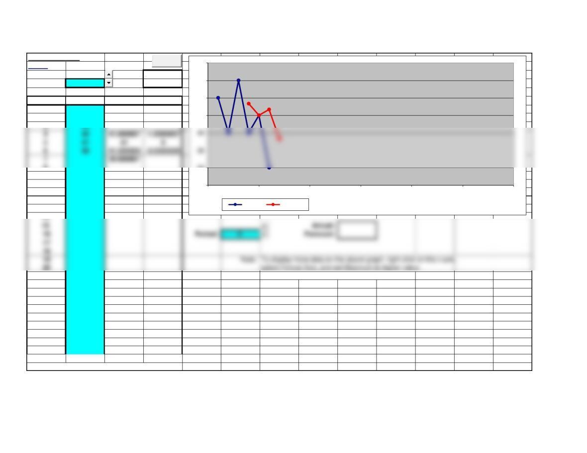
Example 1
Forecast Accuracy Notes
<Back
Forecast 1
MSE = 10.8571429 MSE =
MAPE = 1.2837% MAPE =
Period Actual Forecast 1 Error % Error
1217 215 2 0.92%
2213 216 -3 -1.41%
3216 215 1 0.46%
4210 214 -4 -1.90%
5213 211 2 0.94%
6219 214 5 2.28%
7216 217 -1 -0.46%
8212 216 -4 -1.89%
9
10
11
12
13
19
20 Note: To display more data on the above graph, right click on the x-axis,
22
23
24
25
26
27
28
29
30
31
32
33
209
213
214
215
216
219
220
0 5 10 15 20 25 30
Period
Forecast 1 Series4
Clear
Page 69
Example 1
34
35
36
Page 70
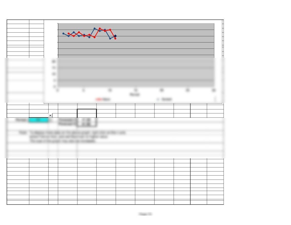
Example 2
Moving Average
<Back
MAD = 1.67
Periods = 3 MSE = 6.94
Period Actual Forecast Error
142 #N/A
240 #N/A
8#N/A
9#N/A
10 #N/A
11 #N/A
12 #N/A
13 #N/A
21 #N/A The size of the graph may also be increased.
22 #N/A
23 #N/A
24 #N/A
25 #N/A
26 #N/A
27 #N/A
28 #N/A
29 #N/A
30 #N/A
Note: rows deleted from template for this example.
37
38
41
42
43
44
0 5 10 15 20 25 30
Period
Actual Forecast
Clear
Page 71
343 #N/A
440 41.666667 -1.6666667
541 41 0
638 41.333333 -3.3333333

Example 4
Forecast Accuracy Notes
<Back
Naive MovingAve ExpSmooth
MAD = 3 MAD = 2.33333333 MAD = 2.4479413
MSE = 14.8888889 MSE = 11.4375 MSE = 8.2101726
MAPE = 7.2450% MAPE = 5.6416% MAPE = 5.8882%
Period Actual Naive Error % Error MovingAve Error % Error ExpSmooth Error % Error
142 #N/A
240 42 -2 -5.00% 42 -2 -5.00%
343 40 3 6.98% 41 2 4.65% 41.8 1.2 2.79%
440 43 -3 -7.50% 41.5 -1.5 -3.75% 41.92 -1.92 -4.80%
14
15
16
17
18
21
22
23
24
25
26
27
28
29
30
31
32
33
34
35
36
Note: rows deleted from template for this example.
Clear
Page 72
541 40 1 2.44% 41.5 -0.5 -1.22% 41.728 -0.728 -1.78%
639 41 -2 -5.13% 40.5 -1.5 -3.85% 41.6552 -2.6552 -6.81%
746 39 7 15.22% 40 6 13.04% 41.38968 4.61032 10.02%
844 46 -2 -4.55% 42.5 1.5 3.41% 41.850712 2.149288 4.88%
945 44 1 2.22% 45 0 0.00% 42.0656408 2.9343592 6.52%
12
13
Example 4
Actual: 40.00
Forecast 1: 38.00
40.00
25
30
35
40
45
50
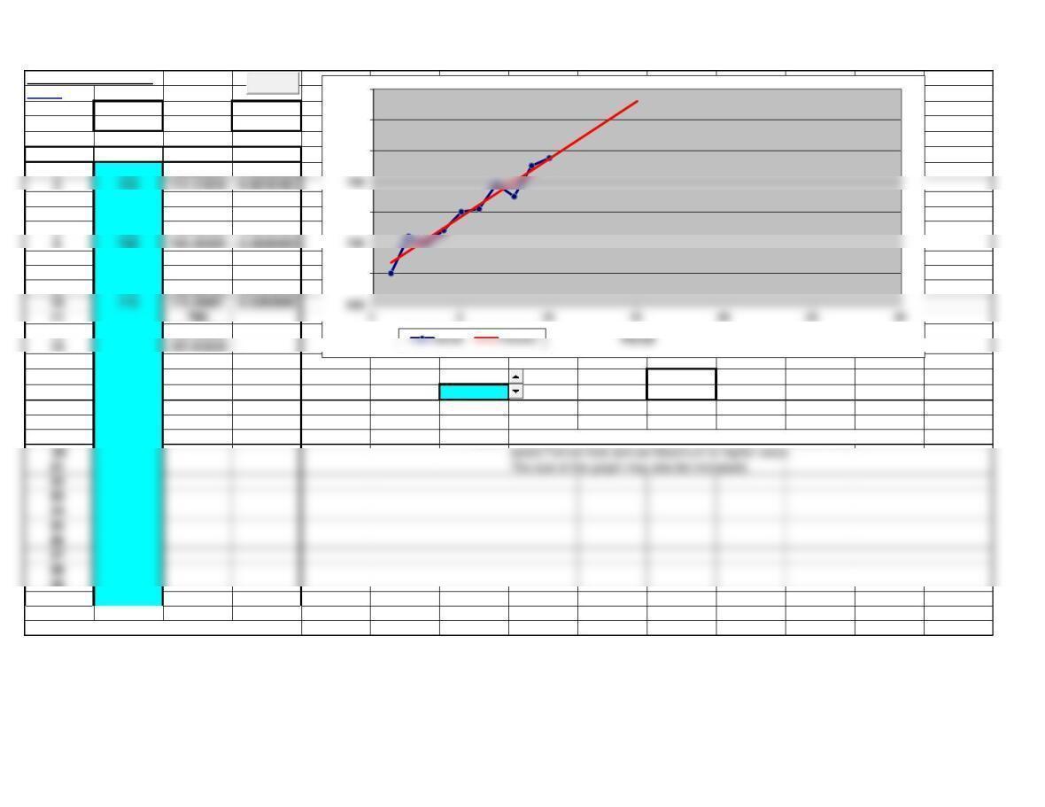
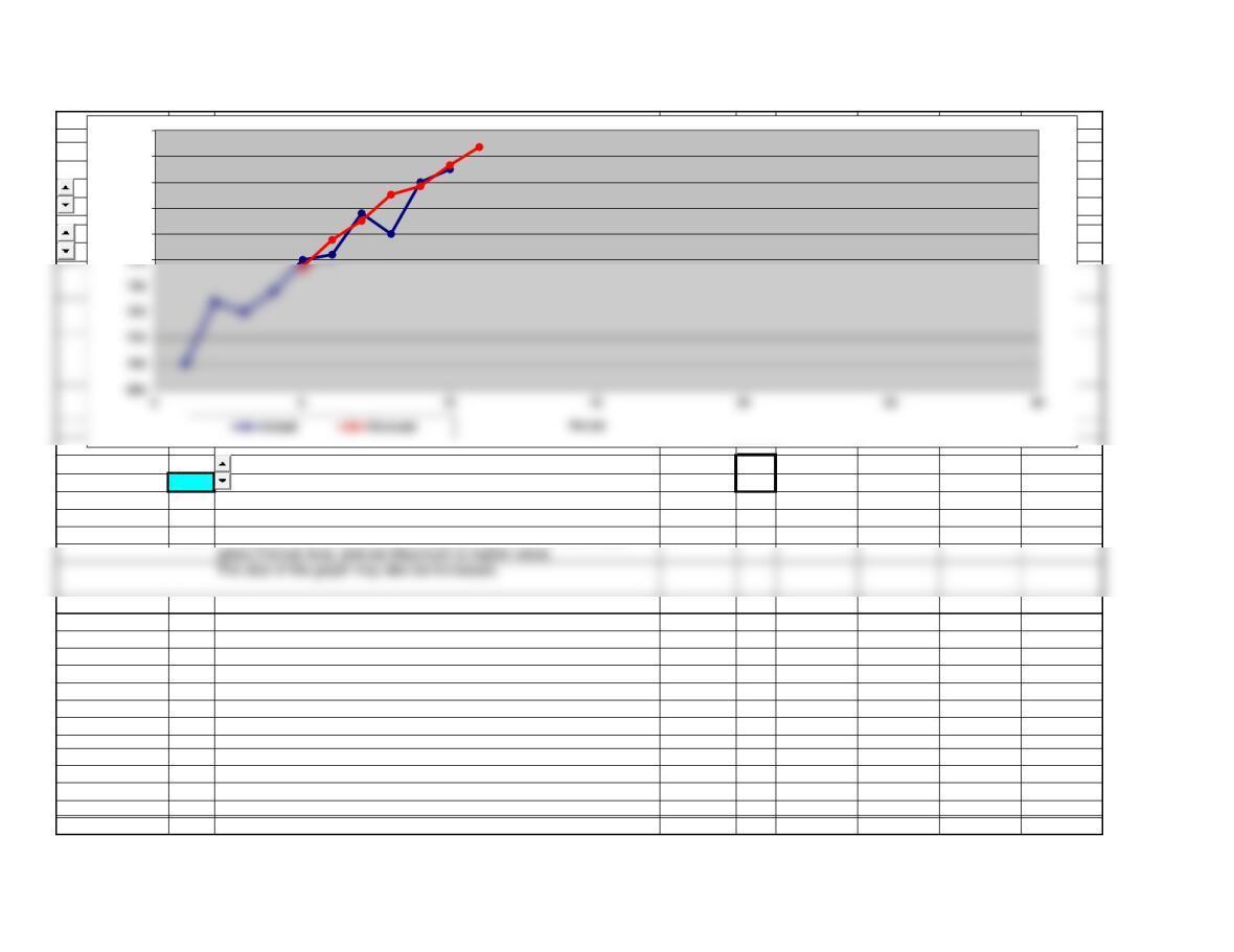
Example 5
Linear Trend Equation
<Back
Slope = 7.5091 MAD = 4.44
Intercept = 699.4 MSE = 32.91
Period Actual Forecast Error
1700 706.90909 -6.9090909 1
3720 721.92727 -1.9272727 3
4728 729.43636 -1.4363636 4
5740 736.94545 3.0545455 5
7758 751.96364 6.0363636 7
8750 759.47273 -9.4727273 8
9770 766.98182 3.0181818 9
12 789.50909
13 797.01818
14 804.52727
15 812.03636 Actual: #N/A
16 #N/A Period: 0 Forecast: #N/A
17 #N/A
18 #N/A
19 #N/A Note: To display more data on the above graph, right click on the x-axis,
20 #N/A select Format Axis and set Maximum to higher value.
21 #N/A The size of the graph may also be increased.
22 #N/A
23 #N/A
24 #N/A
25 #N/A
26 #N/A
27 #N/A
28 #N/A
29 #N/A
30 #N/A
Note: rows deleted from template for this example.
700
740
780
800
820
Clear
Page 74
2724 714.41818 9.5818182 2
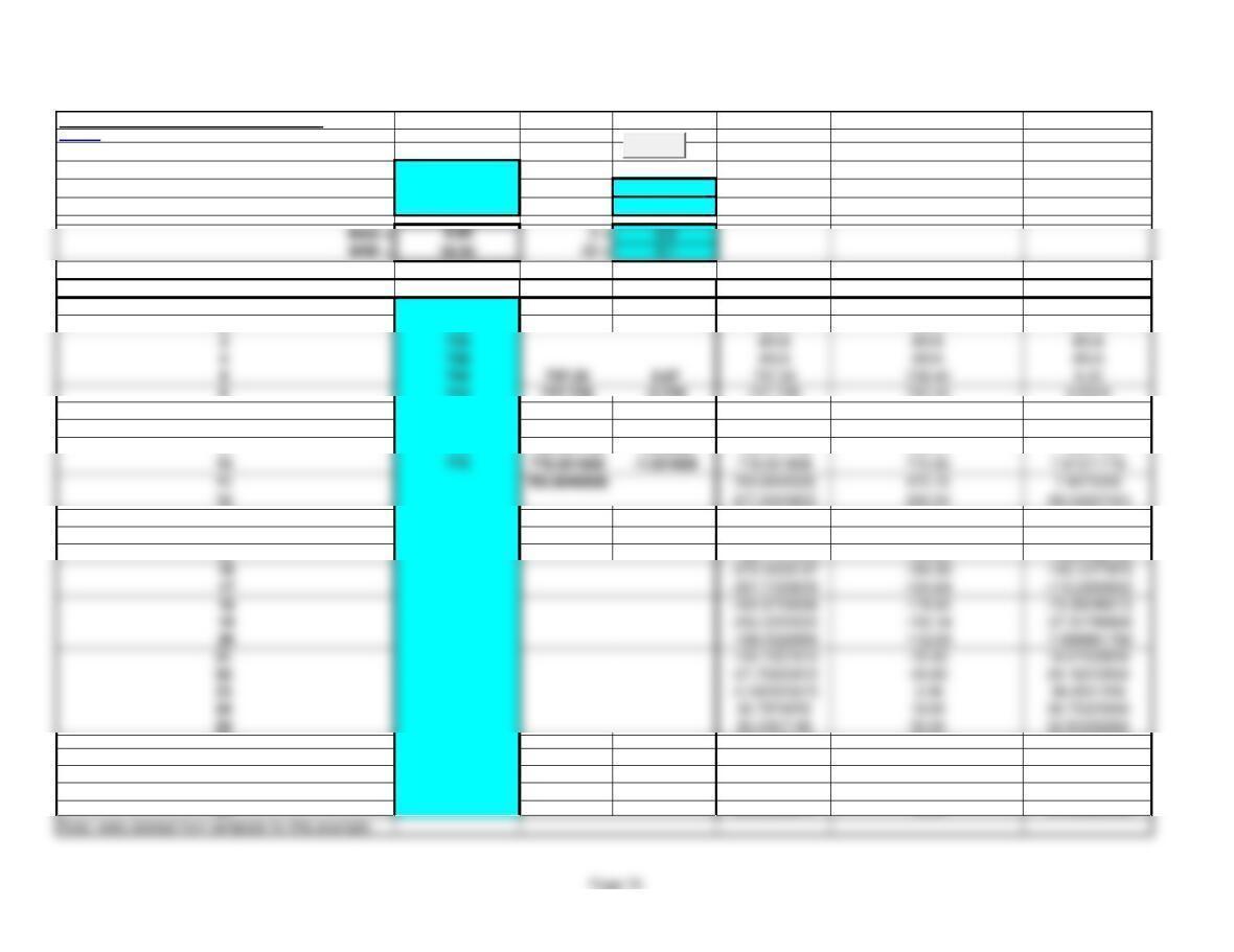
Example 6
Trend Adjusted Exponential Smoothing
<Back
Model Initialization:
Period = 5
Forecast = 737.33 a = 0.4
Trend = 9.33 Da = 0.1
Period Actual Forecast Error TAF S T
1700 #N/A #N/A #N/A #N/A
2724 #N/A #N/A #N/A #N/A
3720 #N/A #N/A #N/A #N/A
4728 #N/A #N/A #N/A #N/A
5740 737.33 2.67 737.33 738.40 9.33
6742 747.728 -5.728 747.728 745.44 9.6504
7758 755.0872 2.9128 755.0872 756.25 8.96304
8750 765.21536 -15.21536 765.21536 759.13 9.312576
9770 768.441792 1.558208 768.441792 769.07 7.4867328
12 #N/A 477.6503823 286.59 -86.54507551
13 #N/A 200.0451539 120.03 -143.8631214
14 #N/A -23.83602905 -14.30 -167.8685399
15 #N/A -182.1701573 -109.30 -165.0082164
21 #N/A -120.7227615 -72.43 14.67539818
22 #N/A -57.75825872 -34.65 29.16212956
24 #N/A 32.7974252 19.68 36.75225969
25 #N/A 56.4307148 33.86 32.81656866
26 #N/A 66.67499754 40.00 26.04488288
27 #N/A 66.04988141 39.63 18.04388318
28 #N/A 57.67381203 34.60 10.11789741
29 #N/A 44.72218463 26.83 3.197039967
30 #N/A 30.03035074 18.02 -2.169622188
Clear
Example 6
Actual: #N/A
Period: 0 Forecast: #N/A
Note: To display more data on the above graph, right click on the x-axis,
750
760
770
780
790
Page 76

Trend and Seasonal
<Back Slope = 7.5
Intercept = 124
Number of “seasons” = 4
Season Index
2 1.1
3 0.75
4 0.95
Period Season Trend Index Forecast Trend: #N/A
1 1 131.5 1.2 157.8 Index: #N/A
2 2 139 1.1 152.9 Period: 0 Forecast: #N/A
10 2199 1.1 218.9
11 3 206.5 0.75 154.875
12 4214 0.95 203.3
13 1 221.5 1.2 265.8
14 2229 1.1 251.9
15 3 236.5 0.75 177.375
16 4244 0.95 231.8
17 1 251.5 1.2 301.8
18 2259 1.1 284.9
0
50
100
250
300
350
0 5 10 15 20 25 30
Period
Trend Forecast
Clear
1 1.2

22 #N/A #N/A
23 #N/A #N/A
24 #N/A #N/A
25 #N/A #N/A
26 #N/A #N/A
27 #N/A #N/A
28 #N/A #N/A
29 #N/A #N/A
30 #N/A #N/A
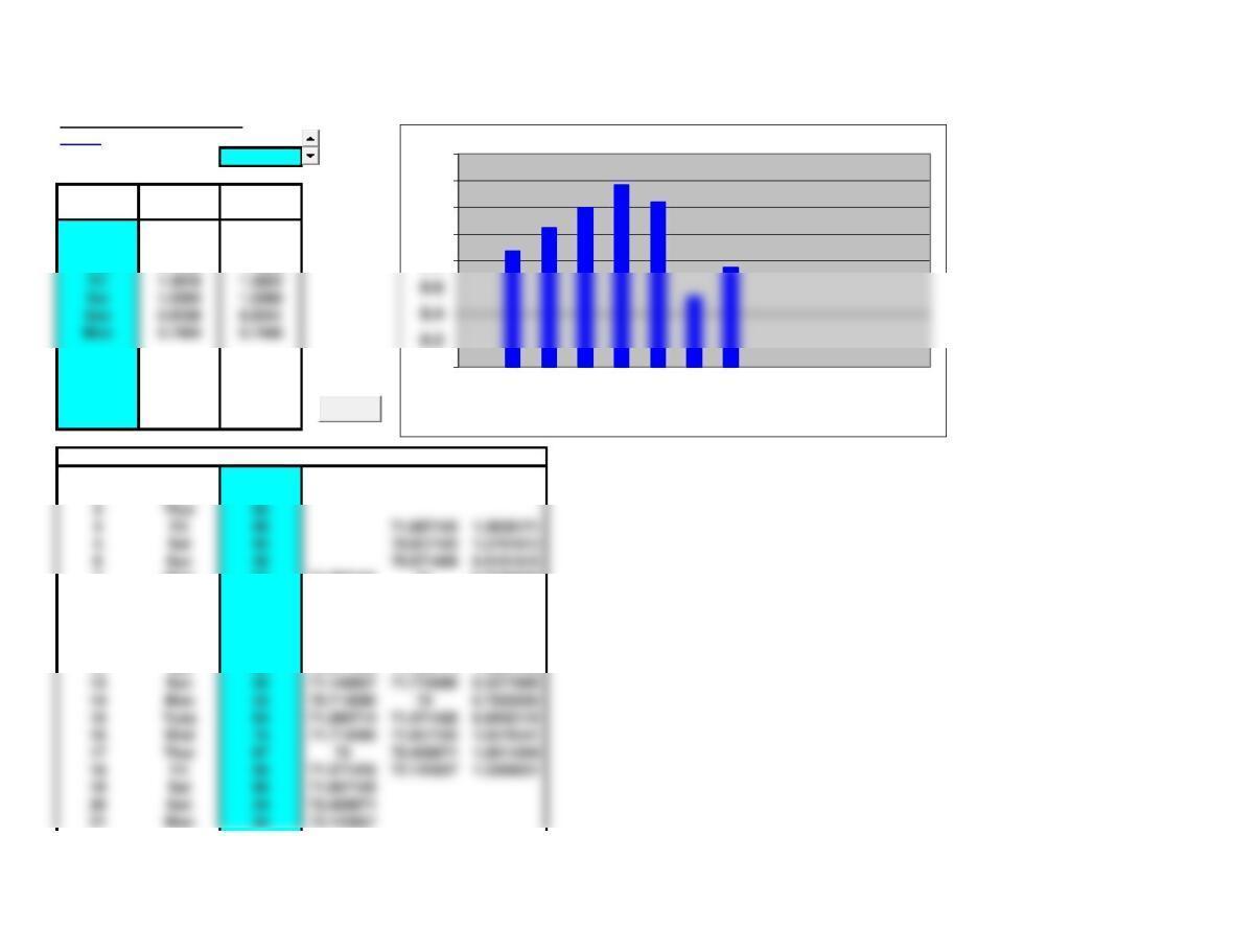
Compute Seasonal Indexes
<Back
Number of “seasons” = 7
Season Average Standard
Index Index
Tues 0.8688 0.8690 season season
Wed 1.0460 1.0463 Tues Mon
Thur 1.1980 1.1983 season season
Fri 0
season season
Sat 0
season season
Sun 0
Period Season Actual MA Center Index
1 Tues 67 #N/A #N/A
2 Wed 75 #N/A #N/A
7 Mon 55 71.857143 71 0.7746479
8 Tues 60 70.857143 71.142857 0.8433735
9 Wed 73 70.571429 70.571429 1.034413
10 Thur 85 71 71.142857 1.1947791
11 Fri 99 71.142857 70.714286 1.4
12 Sat 86 70.571429 71.285714 1.2064128
17 Thur 87 72 72.428571 1.2011834
18 Fri 96 71.571429 72.142857 1.3306931
19 Sat 88 71.857143 #N/A
0
0.8
1
1.2
1.4
1.6
Tues
Wed
Thur
Fri
Sat
Sun
Mon
Clear
Mon 0.7484 0.7486 season season

22 Tues #N/A #N/A
23 Wed #N/A #N/A
24 Thur #N/A #N/A
25 Fri #N/A #N/A
29 Tues #N/A #N/A
30 Wed #N/A #N/A