Unlock document.
This document is partially blurred.
Unlock all pages and 1 million more documents.
Get Access
CHAPTER 3
Decision Analysis
TEACHING SUGGESTIONS
Teaching Suggestion 3.1: Using the Steps of the Decision-Making Process.
The six steps used in decision theory are discussed in this chapter. Students can be asked to
describe a decision they made in the last semester, such as buying a car or selecting an
apartment, and describe the steps that they took. This will help in getting students involved in
decision theory. It will also help them realize how this material can be useful to them in making
important personal decisions.
Teaching Suggestion 3.2: Importance of Defining the Problem and Listing All Possible
Alternatives.
Clearly defining the problem and listing the possible alternatives can be difficult. Students can be
Teaching Suggestion 3.3: Categorizing Decision-Making Types.
Decision-making types are discussed in this chapter; decision making under certainty, risk, and
Teaching Suggestion 3.4: Starting the EVPI Concept.
The material on the expected value of perfect information (EVPI) can be started with a

Teaching Suggestion 3.5: Starting the Decision-Making Under Uncertainty Material.
The section on decision-making under uncertainty can be started with a discussion of optimistic
versus pessimistic decision makers. Students can be shown how maximax is an optimistic
approach, while maximin is a pessimistic decision technique. While few people use these
techniques to solve real problems, the concepts and general approaches are useful.
Teaching Suggestion 3.6: Decision Theory and Life-Time Decisions.
This chapter investigates large and complex decisions. During one’s life, there are a few very
Teaching Suggestion 3.7: Popularity of Decision Trees Among Business Executives.
Stress that decision trees are not just an academic subject; they are a technique widely used by
Teaching Suggestion 3.8: Importance of Accurate Tree Diagrams.
Developing accurate decision trees is an important part of this chapter. Students can be asked to
diagram several decision situations. The decisions can come from the end-of-chapter problems,
the instructor, or from student experiences.
Teaching Suggestion 3.9: Diagramming a Large Decision Problem Using Branches.
Some students are intimidated by large and complex decision trees. To avoid this situation,
Teaching Suggestion 3.10: Using Tables to Perform Bayesian Analysis.
Bayesian analysis can be difficult; the formulas can be hard to remember and use. For many,
ALTERNATIVE EXAMPLES
Alternative Example 3.1: Goleb Transport
George Goleb is considering the purchase of two types of industrial robots. The Rob1
(alternative 1) is a large robot capable of performing a variety of tasks, including welding and
painting. The Rob2 (alternative 2) is a smaller and slower robot, but it has all the capabilities of
Rob1. The robots will be used to perform a variety of repair operations on large industrial
equipment. Of course, George can always do nothing and not buy any robots (alternative 3). The
market for the repair operation could be either favorable (event 1) or unfavorable (event 2).
George has constructed a payoff matrix showing the expected returns of each alternative and the
probability of a favorable or unfavorable market. The data are presented:
EVENT 1
EVENT 2
Probability
0.6
0.4
Alternative 1
50,000
–40,000
Alternative Example 3.2: George Goleb is not confident about the probability of a favorable or
unfavorable market. (See Alternative Example 3.1.) He would like to determine the equally
likely (Laplace), maximax, maximin, criterion of realism (Hurwicz), and minimax regret
decisions. The Hurwicz coefficient should be 0.7. The problem data are summarized below:
EVENT 1
EVENT 2
Probability
0.6
0.4
Alternative 1
50,000
–40,000
Average (alternative 1) = [$50,000 + (–$40,000)]/2
= $5,000
(alternative 1).
The Hurwicz approach uses a coefficient of realism value of 0.7, and a weighted average of
the best and the worst payoffs for each alternative is computed. The results are as follows:
Weighted average (alternative 1) = ($50,000)(0.7)
+ (–$40,000)(0.3)
= $23,000
The minimax regret decision minimizes the maximum opportunity loss. The opportunity loss
table for Goleb is as follows:
Favorable
Unfavorable
Maximum
Alternatives
Market
Market
in Row
Rob1
0
40,000
40,000
Rob2
20,000
20,000
20,000
Alternative Example 3.3: George Goleb is considering the possibility of conducting a survey on
the market potential for industrial equipment repair using robots. The cost of the survey is $5,000.
George has developed a decision tree that shows the overall decision, as in the figure provided.
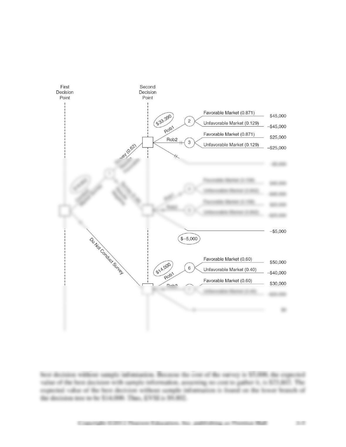
This problem can be solved using EMV calculations. We start with the end of the tree and
work toward the beginning computing EMV values. The results of the calculations are shown in
the tree. The conditional payoff of the solution is $18,802.
Alternative Example 3.4: George (in Alternative Example 3.3) would like to determine the
expected value of sample information (EVSI). EVSI is equal to the expected value of the best
decision with sample information, assuming no cost to gather it, minus the expected value of the

Alternative Example 3.5: This example reveals how the conditional probability values for the
George Goleb examples (above) have been determined. The probability values about the survey
are summarized in the following table:
Results of
Survey
Favorable Market
(FM)
Unfavorable Market
(UM)
Using the values above and the fact that P(FM) = 0.6 and P(UM) = 0.4, we can compute the
Probability revision given a positive survey result
State of
Nature
Conditional
Probability
Prior
Prob.
Joint
Prob.
Posterior
Probability
FM
0.9
0.6
0.54
0.54/0.62 = 0.871
Probability given a negative survey result
State of
Nature
Conditional
Probability
Prior
Prob.
Joint
Prob.
Posterior
Probability
FM
0.1
0.6
0.06
0.06/0.38 = 0.158
Alternative Example 3.6: In the section on utility theory, Mark Simkin used utility theory to
determine his best decision. What decision would Mark make if he had the following utility
values? Is Mark still a risk seeker?
U(–$10,000) = 0.8
U($0) = 0.9
U($10,000) = 1
SOLUTIONS TO DISCUSSION QUESTIONS AND PROBLEMS
3-1. The purpose of this question is to make students use a personal experience to distinguish
between good and bad decisions. A good decision is based on logic and all of the available
3-2. The decision-making process includes the following steps: (1) define the problem, (2) list
the alternatives, (3) identify the possible outcomes, (4) evaluate the consequences, (5) select an
evaluation criterion, and (6) make the appropriate decision. The first four steps or procedures are
common for all decision-making problems. Steps 5 and 6, however, depend on the decision-
making model.
3-3. An alternative is a course of action over which we have complete control. A state of nature
3-4. The basic differences between decision-making models under certainty, risk, and
uncertainty depend on the amount of chance or risk that is involved in the decision. A decision-
3-5. The techniques discussed in this chapter used to solve decision problems under uncertainty
3-6. For a given state of nature, opportunity loss is the difference between the payoff for a
3-7. Alternatives, states of nature, probabilities for all states of nature and all monetary
outcomes (payoffs) are placed on the decision tree. In addition, intermediate results, such as
EMVs for middle branches, can be placed on the decision tree.
3-8. Using the EMV criterion with a decision tree involves starting at the terminal branches of
the tree and working toward the origin, computing expected monetary values and selecting the
3-9. A prior probability is one that exists before additional information is gathered. A posterior
probability is one that can be computed using Bayes’ Theorem based on prior probabilities and
additional information.
3-10. The purpose of Bayesian analysis is to determine posterior probabilities based on prior
probabilities and new information. Bayesian analysis can be used in the decision-making process
3-11. The expected value of sample information (EVSI) is the increase in expected value that
results from having sample information. It is computed as follows:
3-12. The expect value of sample information (EVSI) and the expected value of perfect
3-13. The overall purpose of utility theory is to incorporate a decision maker’s preference for
risk in the decision-making process.
3-14. A utility function can be assessed in a number of different ways. A common way is to use
a standard gamble. With a standard gamble, the best outcome is assigned a utility of 1, and the
worst outcome is assigned a utility of 0. Then, intermediate outcomes are selected and the
3-15. When a utility curve is to be used in the decision-making process, utility values from the
3-16. A risk seeker is a decision maker who enjoys and seeks out risk. A risk avoider is a
3-17. a. Decision making under uncertainty.
b. Maximax criterion.

Row
Row
Equipment
Favorable
Unfavorable
Maximum
Minimum
Sub 100
300,000
–200,000
300,000
–200,000
3-18. Using the maximin criterion, the best alternative is the Texan (see table above) because the
worst payoff for this ($–18,000) is better than the worst payoffs for the other decisions.
3-19. a. Decision making under risk—maximize expected monetary value.
b. EMV (Sub 100) = 0.7(300,000) + 0.3(–200,000)
= 150,000
EMV (Oiler J) = 0.7(250,000) + 0.3(–100,000)
3-20. a. The expected value (EV) is computed for each alternative.
EV(stock market) = 0.5(80,000) + 0.5(–20,000) = 30,000
EV(Bonds) = 0.5(30,000) + 0.5(20,000) = 25,000

3-21. The opportunity loss table is
Alternative
Good Economy
Poor Economy
Stock Market
0
43,000
3-22. a.
Market
Alternative
Condition
Good
Fair
Poor
EMV
Stock market
1,400
800
0
880
3-23. a. Expected value with perfect information is 1,400(0.4) + 900(0.4) + 900(0.2) = 1,100;
the maximum EMV without the information is 900. Therefore, Allen should pay at most
EVPI = 1,100 – 900 = $200.
b. Yes, Allen should pay [1,100(0.4) + 900(0.4) + 900(0.2)] – 900 = $80.
3-24. a. Opportunity loss table
Strong
Fair
Poor
Max.
Market
Market
Market
Regret
Large
0
19,000
310,000
310,000
b. Minimax regret decision is to build medium.
3-25. a.
Stock
Demand
(Cases)
(Cases)
11
12
13
EMV
11
385
385
385
385
b. Stock 11 cases.
c. If no loss is involved in excess stock, the recommended course of action is to stock 13
cases and to replenish stock to this level each week. This follows from the following
decision table.
Stock
Demand
(Cases)
(Cases)
11
12
13
EMV
11
385
385
385
385

3-26.
Manufacture
(Cases)
Demand
(Cases)
6
7
8
9
EMV
6
300
300
300
300
300
7
255
350
350
350
340.5
3-27. Cost of produced case = $5.
Cost of purchased case = $16.
Selling price = $15.
Money recovered from each unsold case = $3.
Supply
Demand(Cases)
(Cases)
100
200
300
EMV
100
100(15) –100(5) =
1000
200(15) – 100(5) –100(16)
= 900
300(15) – 100(5) –200(16)
= 800
900
3-28. a. The table presented is a decision table. The basis for the decisions in the following
questions is shown in the table. The values in the table are in 1,000s.
Decision
MARKET
MAXIMAX
MAXIMIN
EQUALLY
LIKELY
CRIT. OF
REALISM
Alternatives
Good
Fair
Poor
Row
Max.
Row
Min.
Row Ave.
Weighted
Ave.
Small
50
20
–10
50
–10
20
38
MARKET
MINIMAX
Decision
Good
Fair
Poor
Row
Alternatives
Market
Market
Market
Maximum
Small
250
10
0
250
Medium
220
0
10
220

3-29. Note this problem is based on costs, so the minimum values are the best.
a. For a 3-year lease, there are 36 months of payments.
Option 1 total monthly payments: 36($330) = $11,880
Option 2 total monthly payments: 36($380) = $13,680
Option 3 total monthly payments: 36($430) = $15,480
Total cost table
Lease option
36000 miles driven
45000 miles driven
54000 miles driven
Option 1
11,880
15030
18180
Option 3
15,480
15480
15480
b. Optimistic decision: Option 1 because the best (minimum) payoff (cost) for this is 11,800
which is better (lower) than the best payoff for each of the others.
c. Pessimistic decision: Option 3 because the worst (maximum) payoff (cost) for this is 15,480 is
better (lower) than the worst payoff for each of the others.
d. Select Option 2.
EMV(Option 1) = 11,880(0.4) + 15,030(0.3) + 18,180(0.3) = 14,715

3-30. Note that this is a minimization problem, so the opportunity loss is based on the lowest
(best) cost in each state of nature.
Opportunity loss table
Lease option
36000 miles driven
45000 miles driven
54000 miles driven
Option 1
11880 – 11880 = 0
15030 - 13680 = 1350
18180 - 15480 = 2700
3-31. a. P(red) = 18/38; P(not red) = 20/38
b. EMV = Expected win = 10(18/38) + (-10)(20/38) = -0.526
3-32. A $10 bet on number 7 would pay 35($10) = 350 if the number 7 is the winner.
P(number 7) = 1/38; P(not seven) = 37/38
EMV = Expected win = 350(1/38) + (-10)(37/38) = -0.526
3-33. Payoff table with cost of $50,000 in legal fees deducted if suit goes to court and $10,000 in
legal fees if settle.
Win big
Win small
Lose
EMV
Go to court
250000
0
-50000
85000
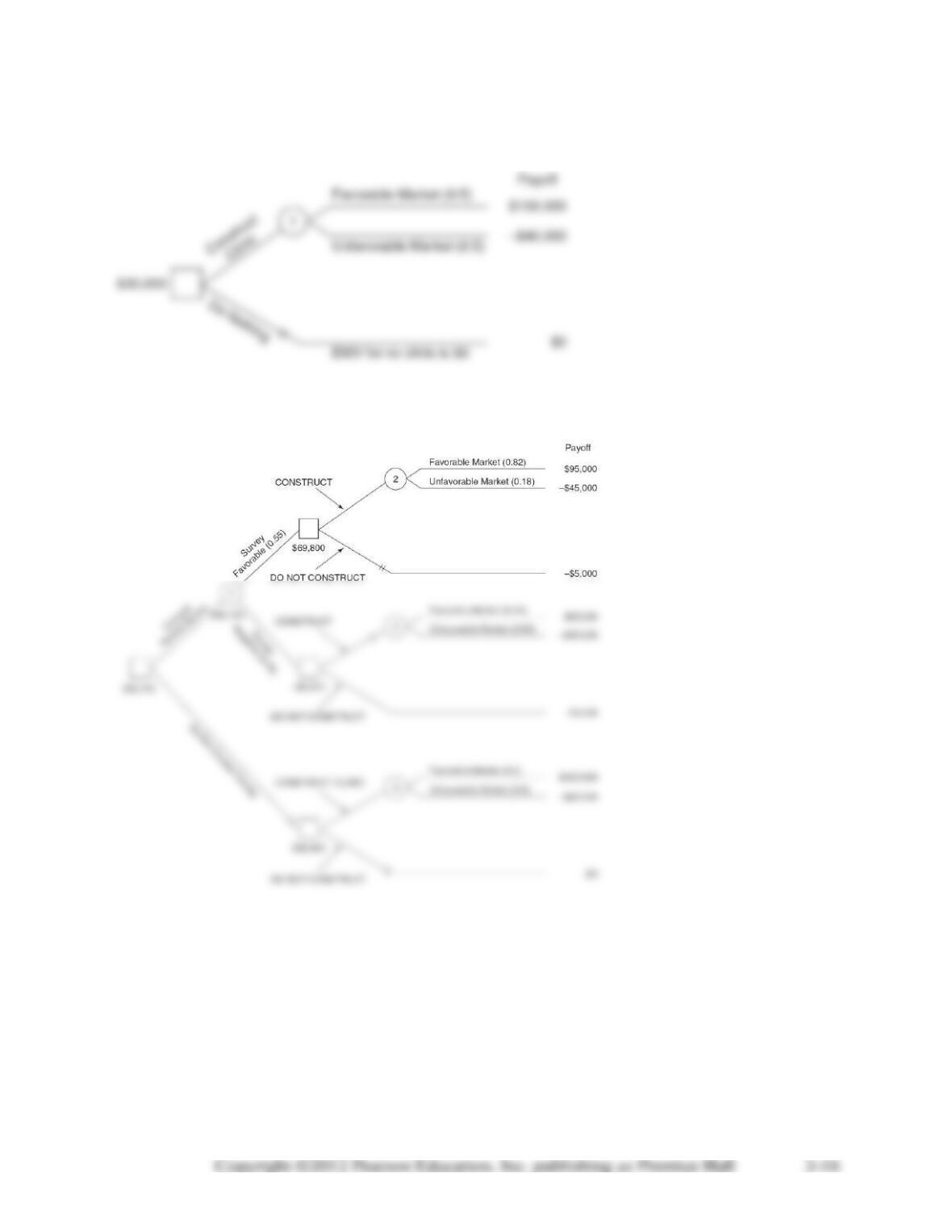
3-34. EMV for node 1 = 0.5(100,000) + 0.5(–40,000) = $30,000. Choose the highest EMV,
therefore construct the clinic.
3-35. a.
b. EMV(node 2) = (0.82)($95,000) + (0.18)(–$45,000)
= 77,900 – 8,100 = $69,800
EMV(node 3) = (0.11)($95,000) + (0.89)(–$45,000)
= 10,450 – $40,050 = –$29,600
3-36.
3-37.
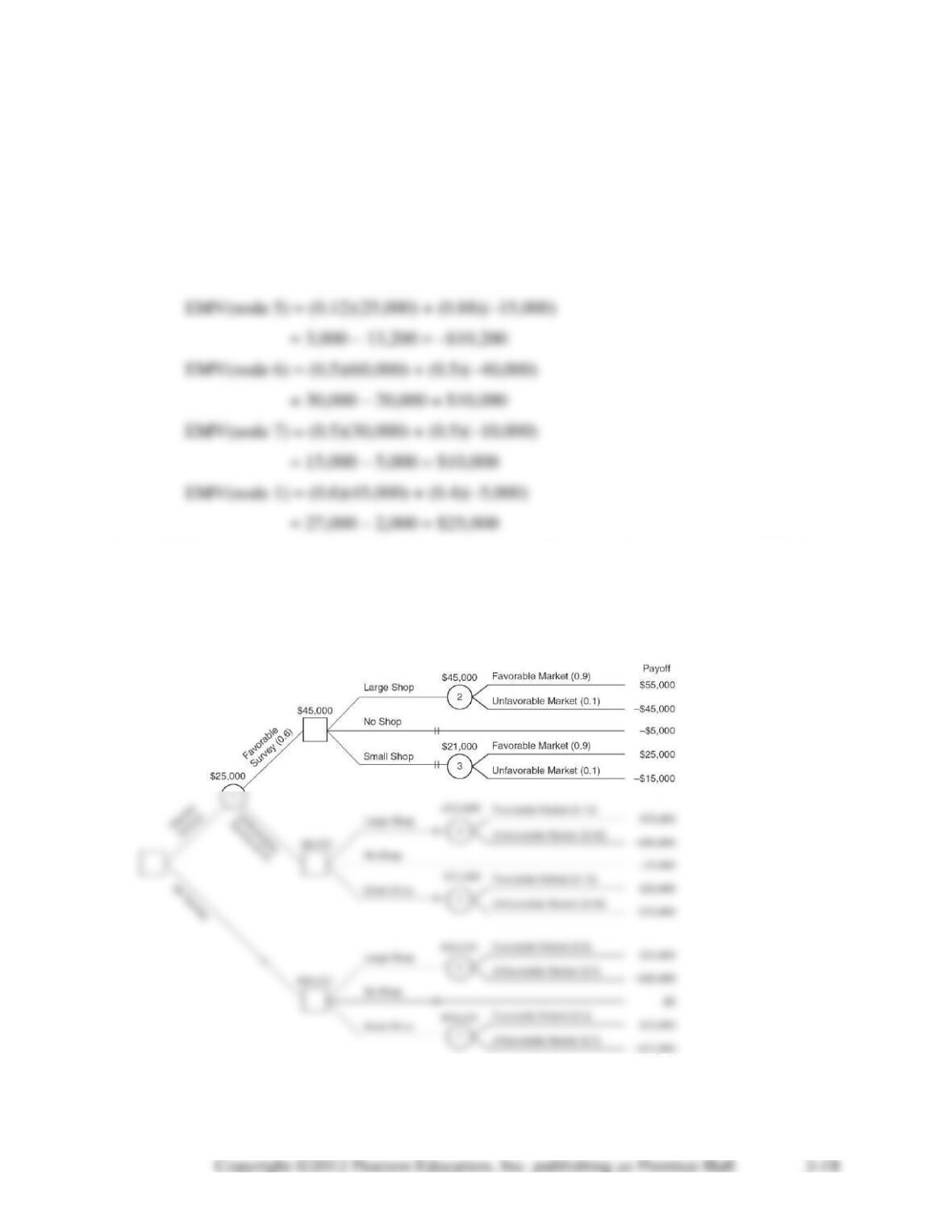
a. EMV(node 2) = (0.9)(55,000) + (0.1)(–$45,000)
= 49,500 – 4,500 = $45,000
EMV(node 3) = (0.9)(25,000) + (0.1)(–15,000)
= 22,500 – 1,500 = $21,000
EMV(node 4) = (0.12)(55,000) + (0.88)(–45,000)
= 6,600 – 39,600 = –$33,000
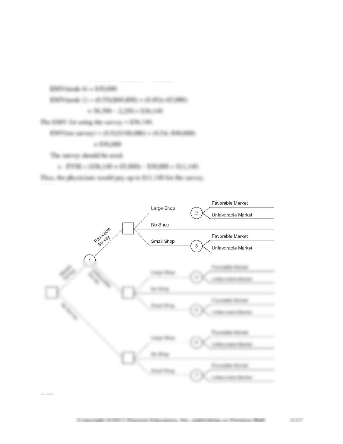
Since EMV(market survey) > EMV(no survey), Jerry should conduct the survey. Since EMV(large
shop | favorable survey) is larger than both EMV(small shop | favorable survey) and EMV(no shop
| favorable survey), Jerry should build a large shop if the survey is favorable. If the survey is
unfavorable, Jerry should build nothing since EMV(no shop | unfavorable survey) is larger than
both EMV(large shop | unfavorable survey) and EMV(small shop | unfavorable survey).
b. If no survey, EMV = 0.5(30,000) + 0.5(–10,000) = $10,000. To keep Jerry from
changing decisions, the following must be true:
EMV(survey) ≥ EMV(no survey)
Let P = probability of a favorable survey. Then,
P[EMV(favorable survey)] + (1 – P) [EMV(unfavorable survey)] ≥ EMV(no survey)
Thus, the probability of a favorable survey could be as low as 0.3. Since the marketing
professor estimated the probability at 0.6, the value can decrease by 0.3 without causing Jerry
to
change his decision. Jerry’s decision is not very sensitive to this probability value.
3-38.

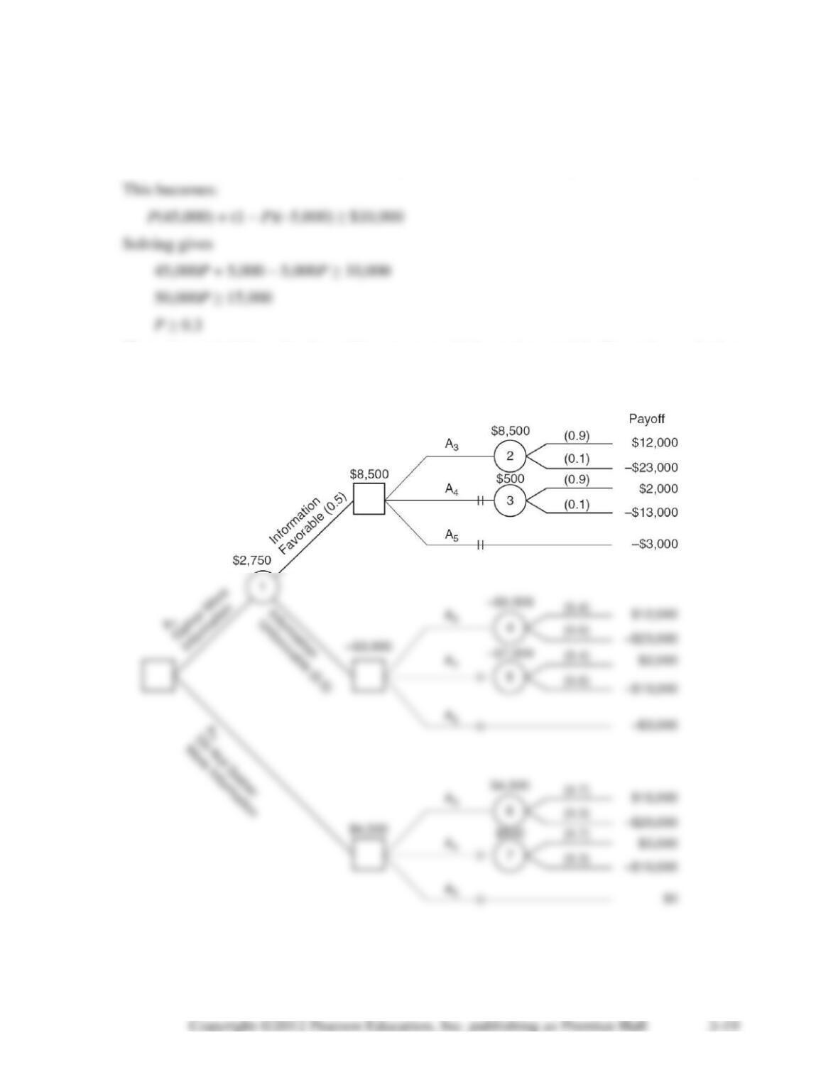
A1: gather more information
A2: do not gather more information
A3: build quadplex
A4: build duplex
A5: do nothing
Decisions: do not gather information; build quadplex.
3-39. I1: favorable research or information
P(S1) = 0.5; P(S2) = 0.5
P(I1 | S1) = 0.8; P(I2 | S1) = 0.2
P(I1 | S2) = 0.3; P(I2 | S2) = 0.7
a. P(successful store | favorable research) = P(S1 | I1)


