CHAPTER 2 REVIEW 2-35
11. log
x36 = 2 12. log
216 = x
13. 10
x = 143.7 14. ex = 503,000
15. log x = 3.105 16. ln x = –1.147
17. (A) y = 4 (B) x = 0 (C) y = 1 (D) x = –1 or 1
(E) y = –2 (F) x = –5 or 5 (2-1)
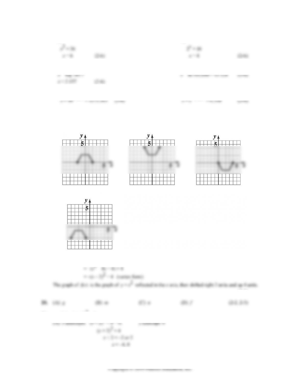
18. (A) (B) (C)
(D)
(2-2)
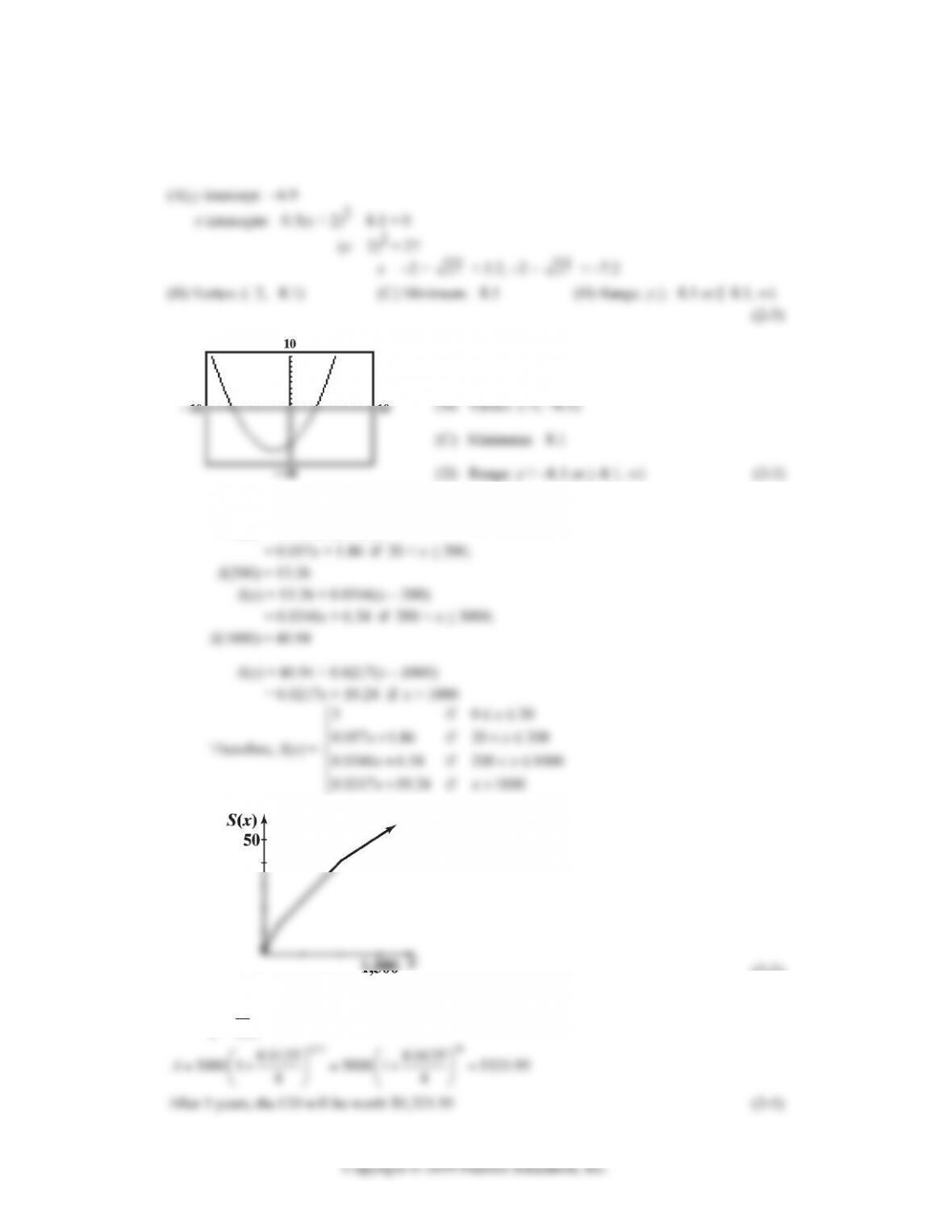
19. f(x) = –x2 + 4x = –(x2 – 4x)
(2-3)
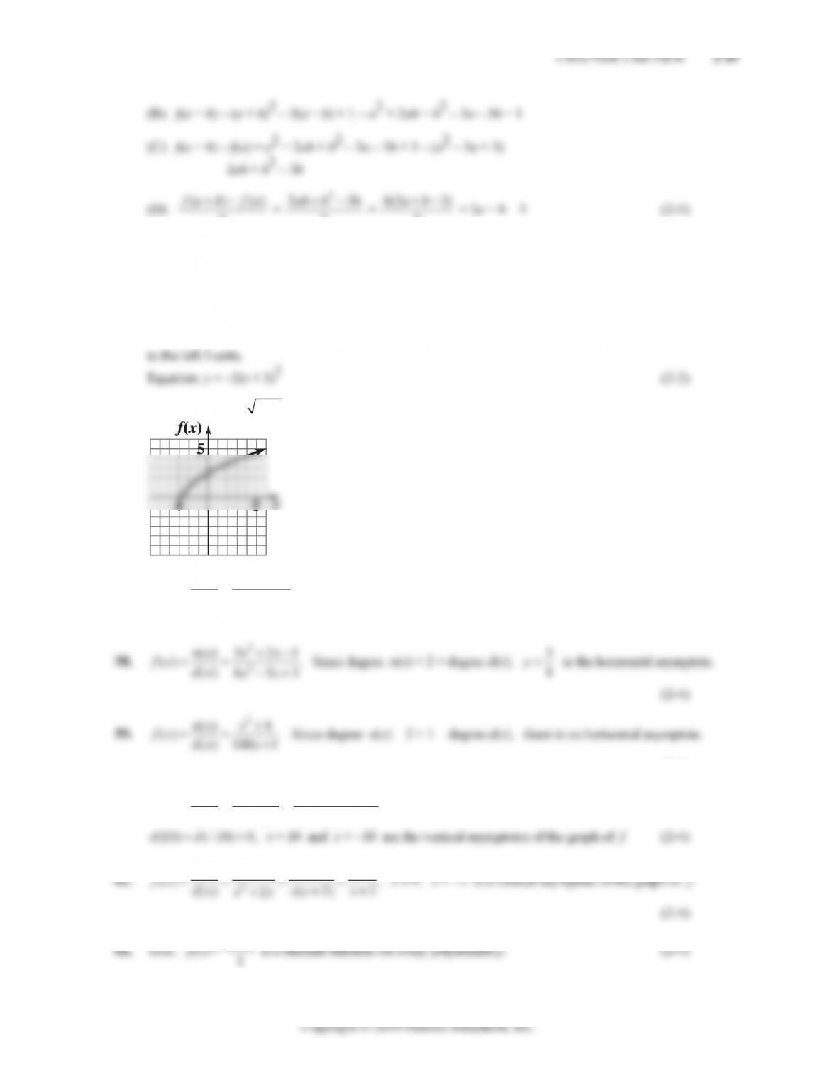
21. y = f(x) = (x + 2)2 4
2-36 CHAPTER 2: FUNCTIONS
Copyright © 2019 Pearson Education, Inc.
(B) Vertex: (2, 4) (C) Minimum: 4 (D) Range: y ≥ 4 or [4, ∞) (2-3)
22. y = 4 – x + 3x2 = 3x2 – x + 4; quadratic function. (2-3)
x
24. y = 74
2
x
x
= 7
2
x
– 2; none of these. (2-1), (2-3)
26. log(x + 5) = log(2x – 3) 27. 2 ln(x – 1) = ln(x2 – 5)
28. 11
93
x
x
29. 2
23xx
ee
21 1
x
x
x
x
30. 2
23
x
x
x
exe 31. 1/3
log 9
x
2
23
x
x
19
3
x
32. log 8 3
x 33. log
9x = 3
2
2
34. x = 3(e1.49) ≈ 13.3113 (2-5) 35. x = 230(10–0.161) ≈ 158.7552 (2-5)
36. log x = –2.0144 37. ln x = 0.3618
2-38 CHAPTER 2: FUNCTIONS
44. f(x) = ex – 1, g(x) = ln(x + 2)
2
-2
Points of intersection:
45. f(x) = 2
50
1x:
3210123
() 510255025105
x
fx
(2-1)
46. f(x) = 2
66
2
x
:
()611226622116
x
fx
(2-1)
For Problems 47–50, f(x) = 5x + 1.
47. f(f(0)) = f(5(0) + 1) = f(1) = 5(1) + 1 = 6 (2-1)
50. f(4 – x) = 5(4 – x) + 1 = 20 – 5x + 1 = 21 – 5x (2-1)
51. f(x) = 3 – 2x
(A) f(2) = 3 – 2(2) = 3 – 4 = –1
52. f(x) = x2 – 3x + 1
Copyright © 2019 Pearson Education, Inc.
(D) ()()
h
h
h
53. The graph of m is the graph of y = |x| reflected in the x axis and shifted 4 units to the right. (2-2)
54. The graph of g is the graph of y = x3 vertically contracted by a factor of 0.3 and shifted up 3 units.
(2-2)
55. The graph of y = x2 is vertically expanded by a factor of 2, reflected in the x axis and shifted
56. Equation: f(x) = 2 3x – 1
(2-2)
57. 2
() 5 4
() .
() 31
nx x
fx dx xx
Since degree n(x) = 1< 2 = degree d(x), y = 0 is the horizontal asymptote.
(2-4)
2
() 3 2 1
nx x x
( ) 100 1
(2-4)
60.
22
2
( ) 100 100
() .
( ) ( 10)( 10)
100
nx x x
fx dx x x
x
Since 2
() 100nx x has no real zeros and
2-40 CHAPTER 2: FUNCTIONS
Copyright © 2019 Pearson Education, Inc.
65. True: let f(x) = bx, (b > 0, b ≠ 1), then the positive x-axis is a horizontal asymptote if 0 < b < 1,
66. True: let f(x) = logbx (b > 0, b ≠ 1). If 0 < b < 1, then the positive y-axis is a vertical asymptote;
(2-2)
(2-2)
70. y = –(x – 4)2 + 3 (2-2, 2-3)
71. f(x) = –0.4x2 + 3.2x + 1.2 = –0.4(x2 – 8x + 16) + 7.6
(2-3)
72.
(A) y intercept: 1.2
x intercepts: –0.4, 8.4
73. log 10π = π log 10 = π
log 2
10 = y is equivalent to log y = log 2
CHAPTER 2 REVIEW 2-41
74. log x log 3 = log 4 log (x + 4)
4
log log
34
x
x
75. ln(2x – 2) – ln(x – 1) = ln x 76. ln(x + 3) – ln x = 2 ln 2
ln 22
1
x
x
= ln x 3
ln x
x
= ln(22)
x
77. log 3x2 = 2 + log 9x 78. ln y = –5t + ln c
log 3x2 – log 9x = 2 ln y – ln c = –5t
2
x
x
x
c = e–5t
x
79. Let x be any positive real number and suppose log1x = y. Then 1y = x.
y = 1, so x = 1, i.e., x = 1 for all positive real numbers x.
80. The graph of y = 3
x
is vertically expanded by a factor of 2, reflected in the x axis, shifted 1 unit to the left
x
2-42 CHAPTER 2: FUNCTIONS
81. G(x) = 0.3x2 + 1.2x – 6.9 = 0.3(x2 + 4x + 4) – 8.1
= 0.3(x + 2)2 – 8.1
82.
(A) y intercept: –6.9
x intercept: –7.2, 3.2
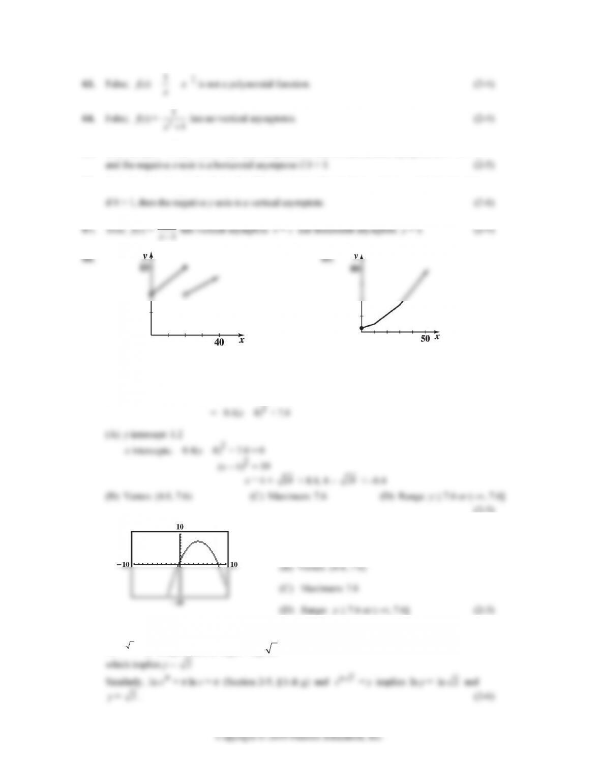
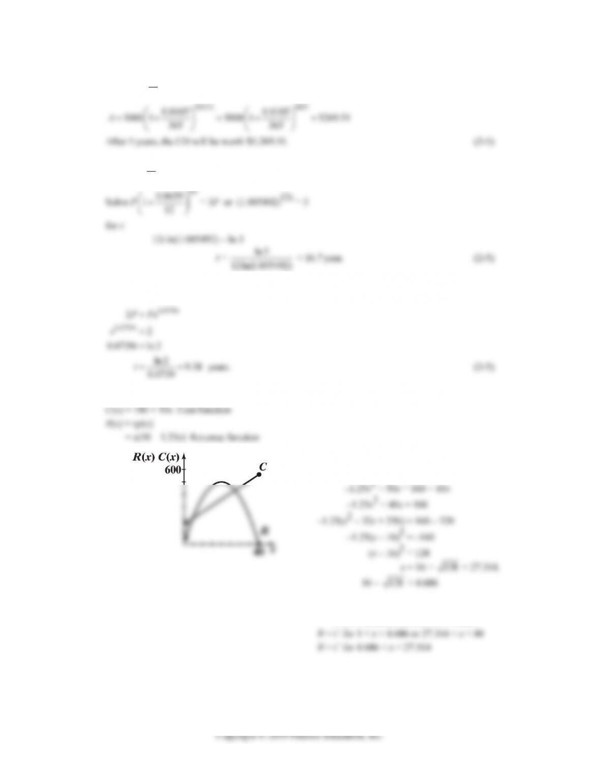
83. (A) S(x) = 3 if 0 ≤ x ≤ 20;
S(x) = 3 + 0.057(x – 20)
0.0346 6.34 if 200 1000
0.0217 19.24 if 1000
xx
xx
(B)
(2-2)
84. 1;
mt
r
AP m
P = 5,000, r = 0.0125, m = 4, t = 5.
CHAPTER 2 REVIEW 2-43
85. 1
mt
r
AP m
; P = 5,000, r = 0.0105, m = 365, t = 5
86. A = P1
mt
r
m
, r = 0.0659, m = 12
12
0.0659
t
87. , 0.0739
rt
APe r. Solve 0.0739
2for .
t
PPe t
0.0739
0.0739
2
2
0.0739 ln 2
ln 2 9.38 years.
0.0739
t
t
PPe
e
t
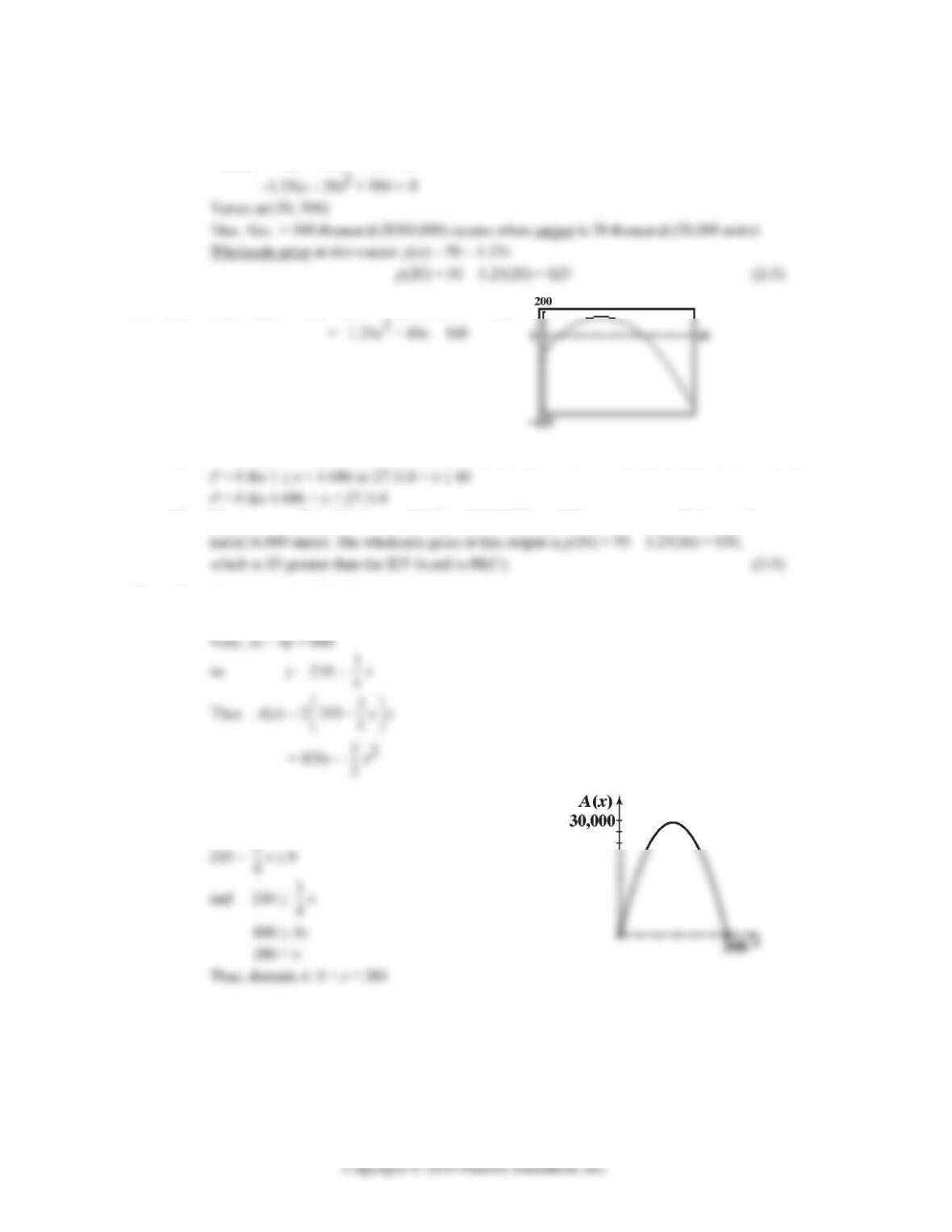
88. p(x) = 50 – 1.25x Price-demand function
(A)
(B) R = C
x(50 – 1.25x) = 160 + 10x
R = C at x = 4.686 thousand units (4,686 units) and
x = 27.314 thousand units (27,314 units)
2-44 CHAPTER 2: FUNCTIONS
(C) Max Rev: 50x – 1.25x2 = R
–1.25(x2 – 40x + 400) + 500 = R
89. (A) P(x) = R(x) – C(x) = x(50 – 1.25x) – (160 + 10x)
(B) P = 0 for x = 4.686 thousand units (4,686 units) and x = 27.314 thousand units (27,314 units)
(C) Maximum profit is 160 thousand dollars ($160,000), and this occurs at x = 16 thousand
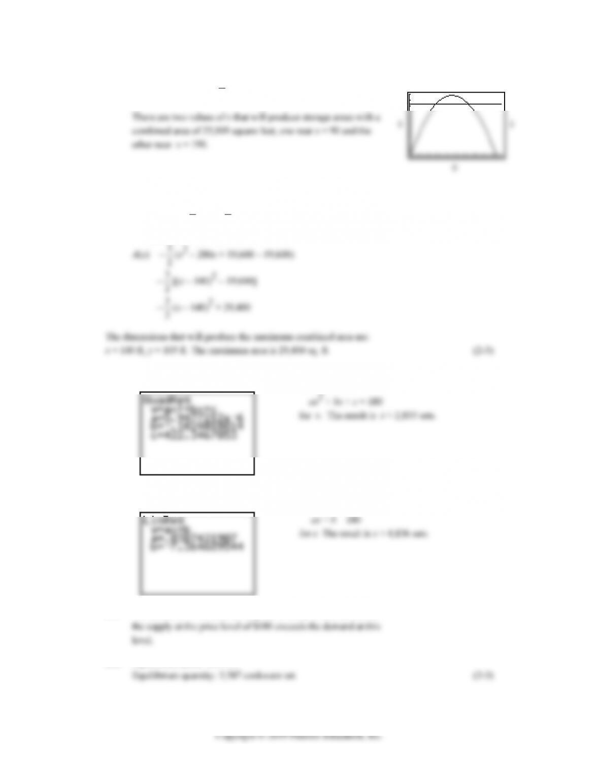
90. (A) The area enclosed by the storage areas is given by
A = (2y)x
(B) Clearly x and y must be nonnegative; the fact
that y ≥ 0 implies
3
(C)
CHAPTER 2 REVIEW 2-45
(D) Graph A(x) = 420x – 3
2x2 and y = 25,000 together.
30,000
(E) x = 86, x = 194
(F) A(x) = 420x – 3
2x2 = – 3
2 (x2 – 280x)
Completing the square, we have
91. (A) Quadratic regression model,
Table 1:
To estimate the demand at price level of $180, we solve
the equation
(B) Linear regression model,
Table 2:
To estimate the supply at a price level of $180, we solve
the equation
(C) The condition is not stable; the price is likely to decrease since
(D) Equilibrium price: $131.59
2-46 CHAPTER 2: FUNCTIONS
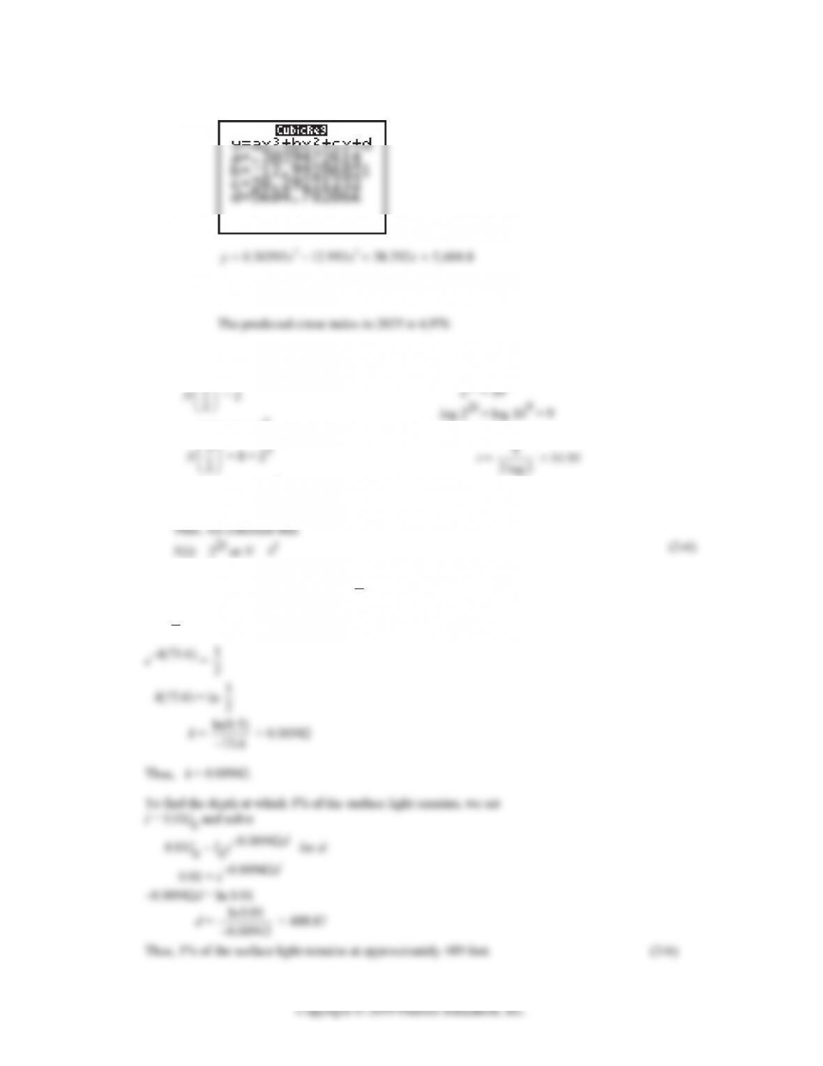
92. (A) Cubic Regression
(B) 32
0.30395(38) 12.993(38) 38.292(38) 5,604.8 4,976y
93.
(A) N(0) = 1
N(1) = 4 = 22
N(2) = 16 = 24
(B) We need to solve:
2t log 2 = 9
Thus, the mouse will die in 15 days.
94. Given I = I0e–kd. When d = 73.6, I = 1
2I0. Thus, we have:
1
2I0 = I0e–k(73.6)