2-1
2 FUNCTIONS
EXERCISE 2-1
2.
4.
6.
8.
10. The table specifies a function, since for each domain value there corresponds one and only one range value.
12. The table does not specify a function, since more than one range value corresponds to a given domain
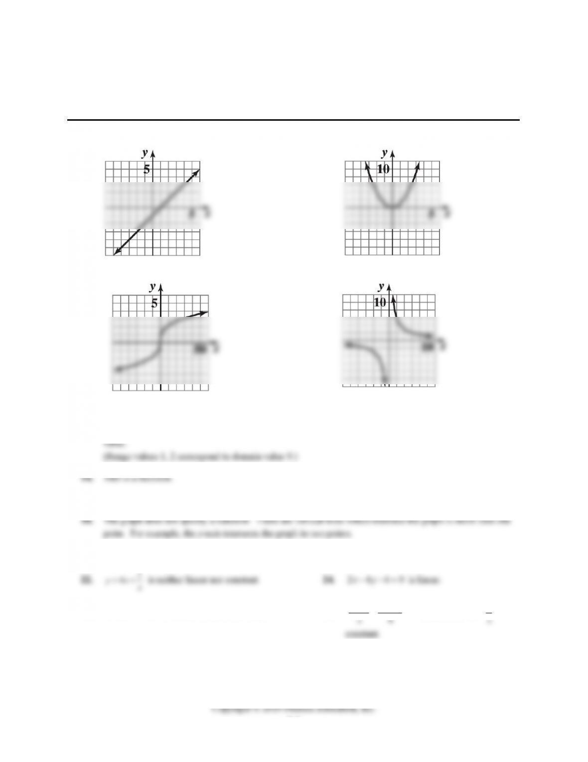
16. The graph specifies a function; each vertical line in the plane intersects the graph in at most one point.
20. The graph does not specify a function.
26. 10xxy is neither linear nor constant. 28. 32 1
yx x
simplifies to 1
y
30.
32.
34.
36.
38. f(x) =
2
2
3
2
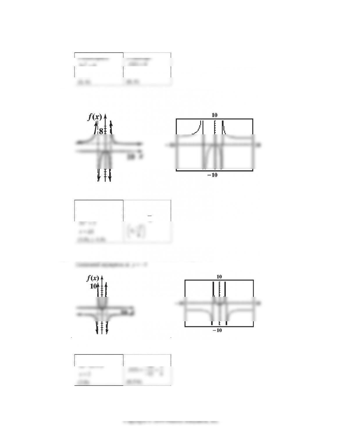
x
x. Since the denominator is bigger than 1, we note that the values of f are between 0 and 3.
Furthermore, the function f has the property that f(–x) = f(x). So, adding points x = 3, x = 4,
x = 5, we have:
x
–
5
–
4
–
3
–
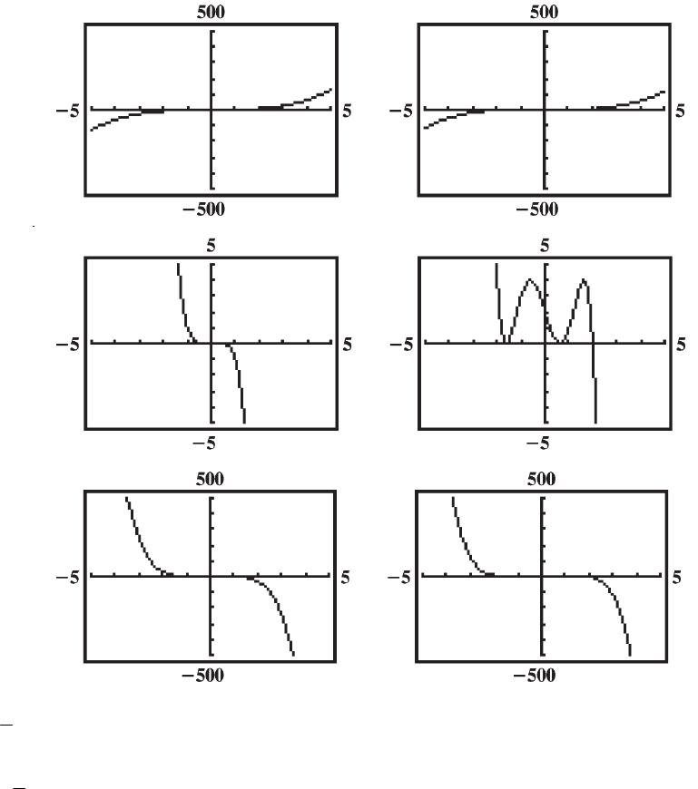
2
–
1 0 1 2 3 4 5
F
x
The sketch is:
40. y = f(4) = 0 42. y = f(–2) = 3
48. Domain: all real numbers. 50. Domain: all real numbers except x = 2.

EXERCISE 2-1 2-3
56. Given ()4xx y. Solving for y we have:
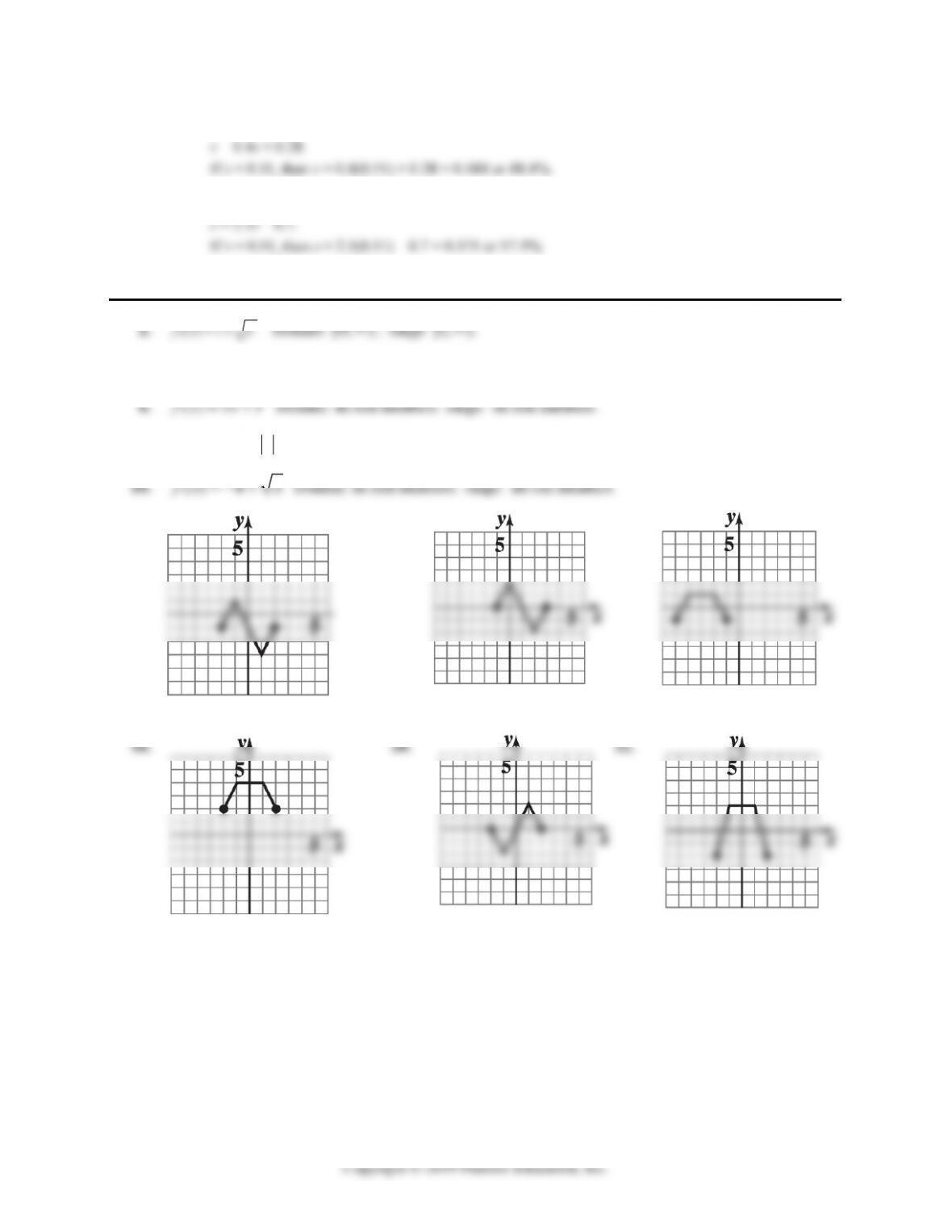
2
24
4and .
x
xy x y
x
58. Given 22.9xy Solving for y we have: 22 2
9 and 9 .yx y x
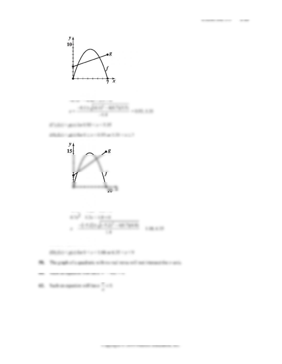
60. Given 30.xy. Solving for y we have: 31/6
and .yxyx
66. 2633
()() 4 4fx x x
70. 22 2 2
(3) () (3) 4 4 5 4 1ffh h hh
76. (A) ( ) 3( )9 339fx h x h x h
78. (A) 2
()3()5()8
fx h x h x h
(B)
22 2
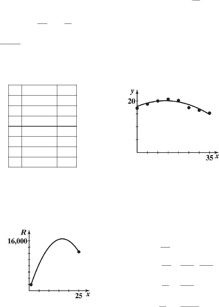
()()363558358
fx h fx x xh h x h x x
80. (A) f(x + h) = x2 + 2xh + h2 + 40x + 40h
82. Given A = l w = 81.
84. Given P = 2
+ 2w = 160 or
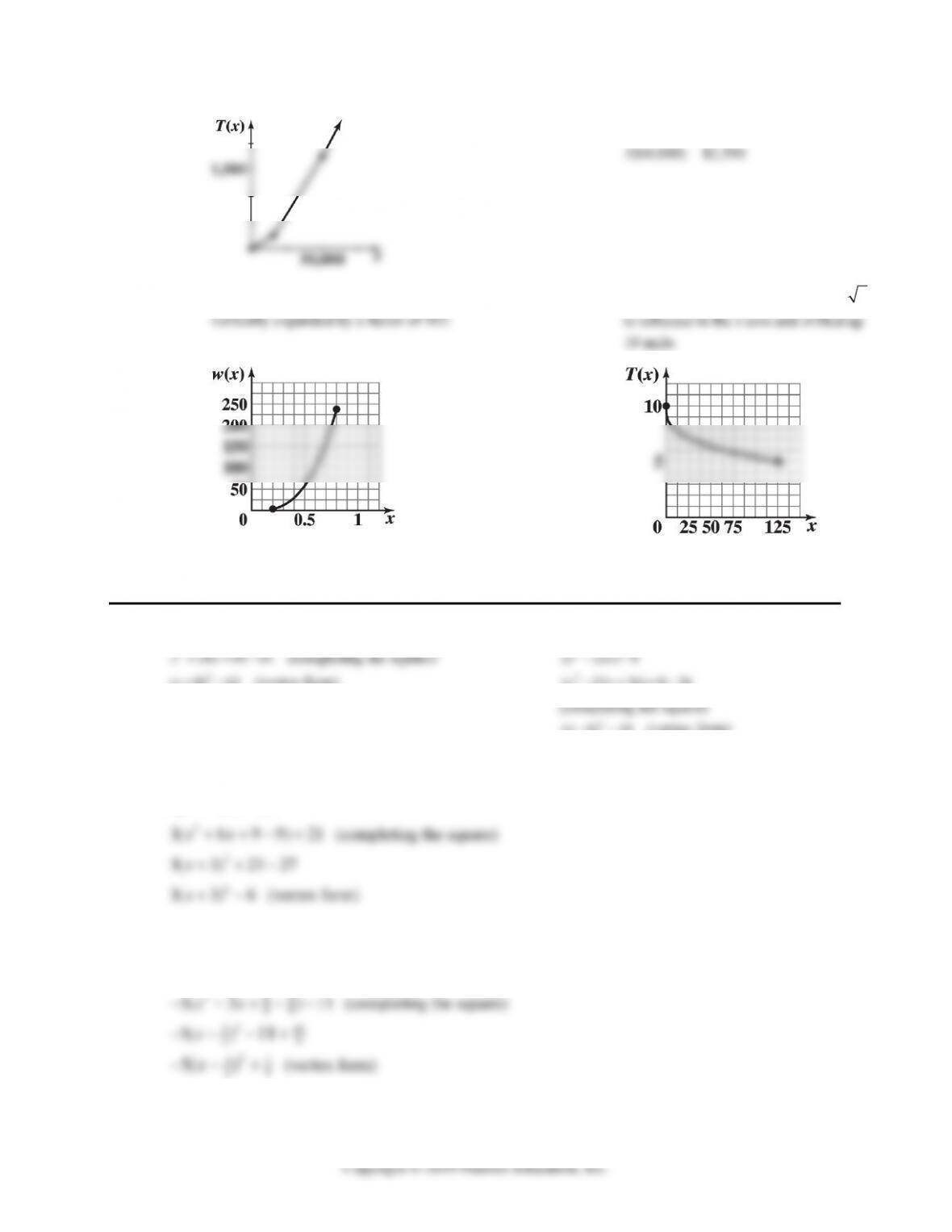
+ w = 80 and
= 80 – w.
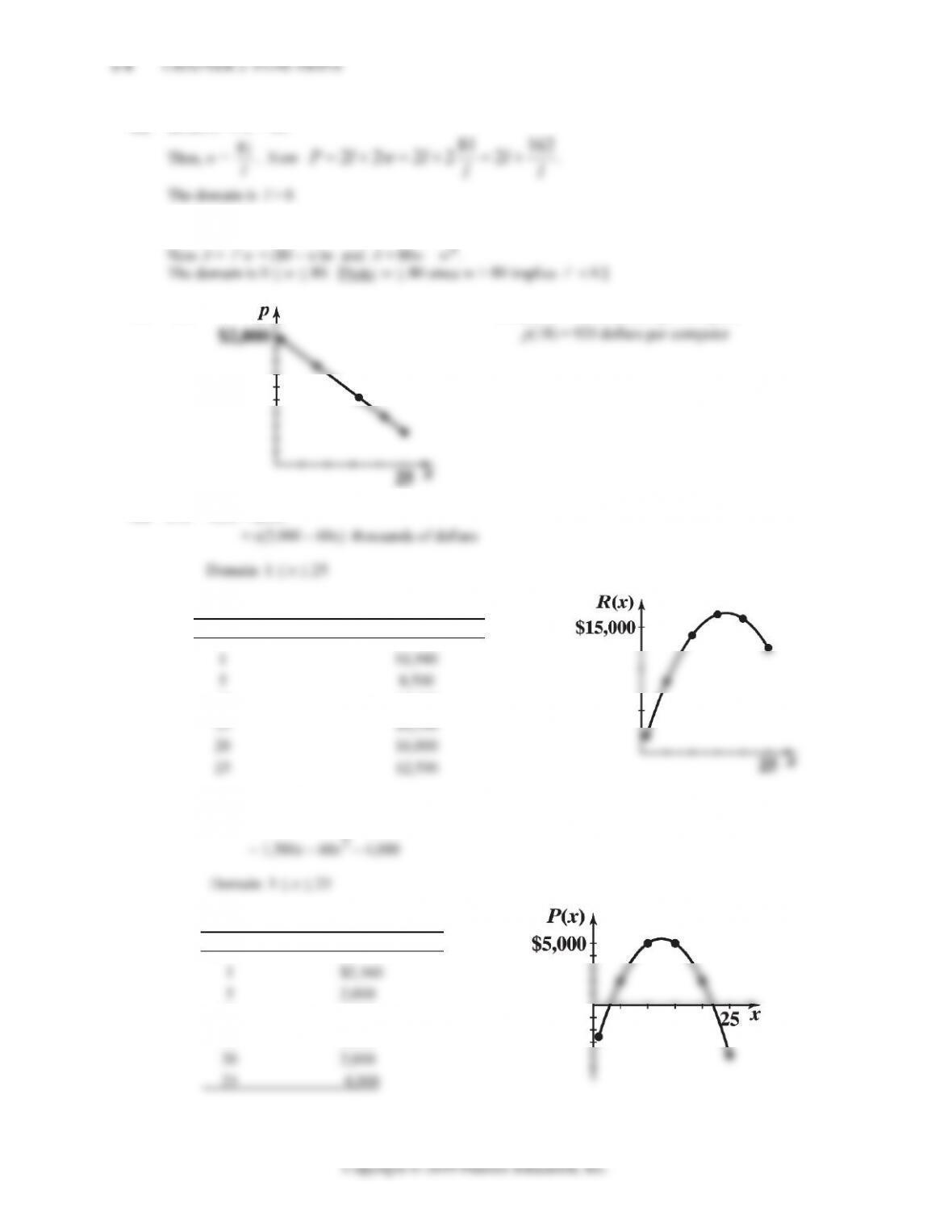
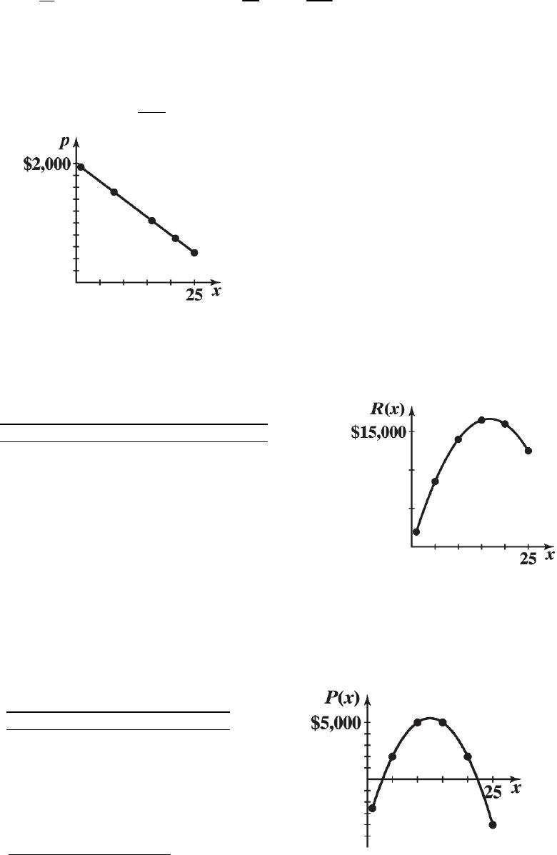
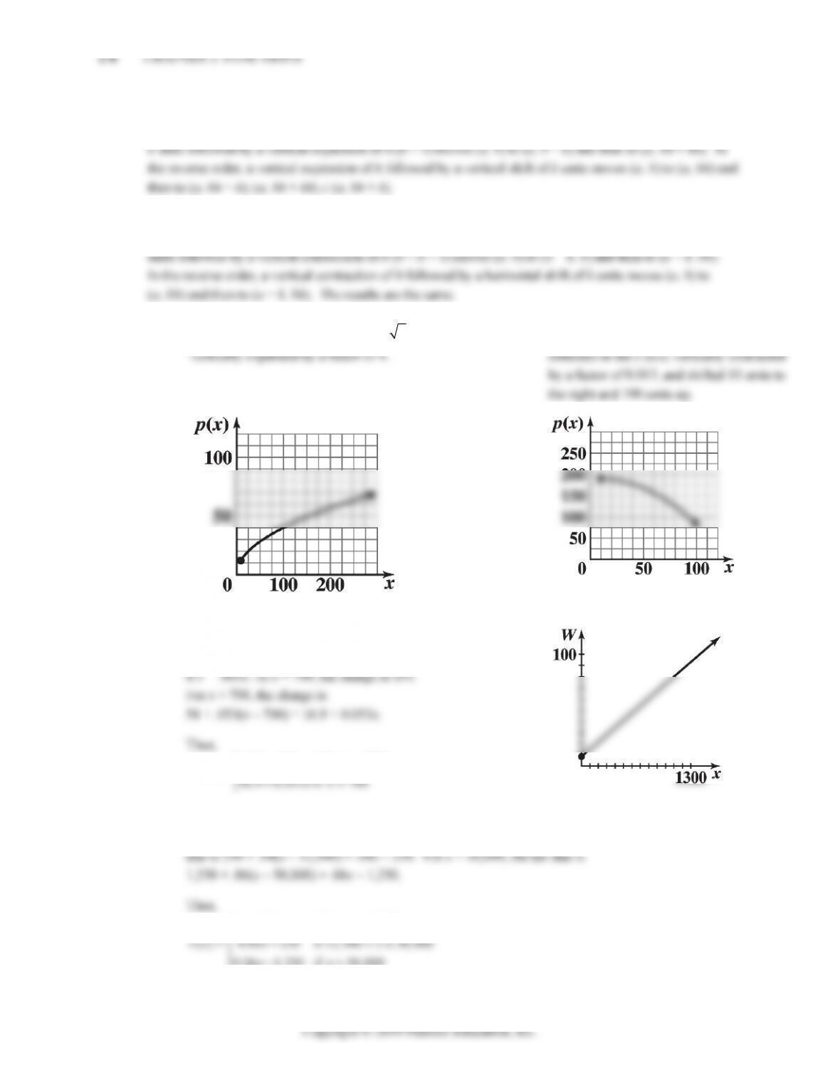
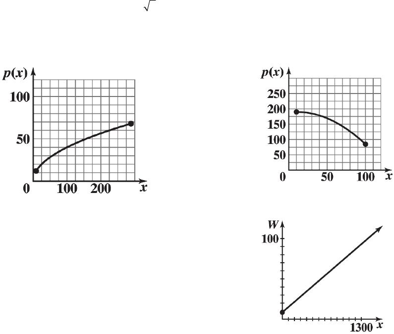
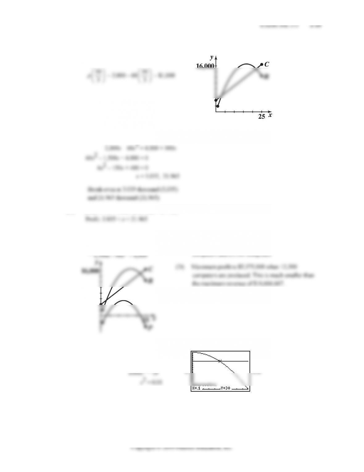
86. (A)
(B) p(11) = 1,340 dollars per computer
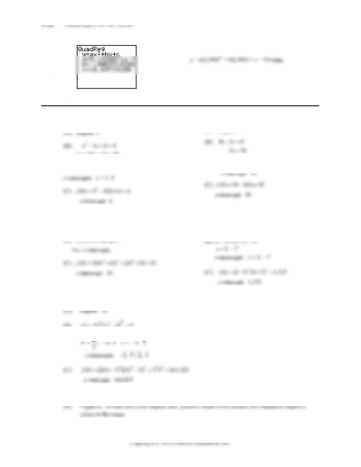
88. (A) R(x) = xp(x)
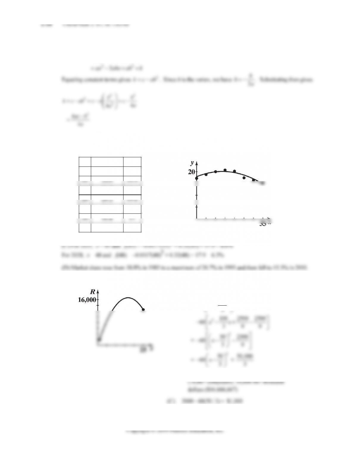
(B) Table 11 Revenue
x(thousands) R(x)(thousands)
10 14,000
(C)
90. (A) P(x) = R(x) – C(x)
= x(2,000 – 60x) – (4,000 + 500x) thousand dollars
(B) Table 13 Profit
x (thousands) P(x) (thousands)
10 5,000
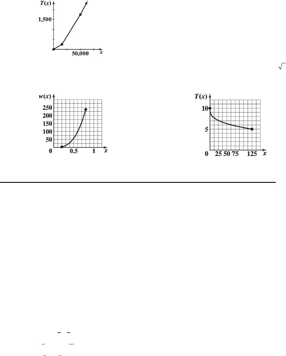
15 5,000
(C)
EXERCISE 2-2 2-5
92. (A) Given 5v – 2s = 1.4. Solving for v, we have:
(B) Solving the equation for s, we have:
EXERCISE 2-2
f
4. 2
() 10fx x Domain: all real numbers; range: [10, ).
8. ( ) 15 20
f
xx Domain: all real numbers; range: (,15].
12.
14.
16.
2-6 CHAPTER 2: FUNCTIONS
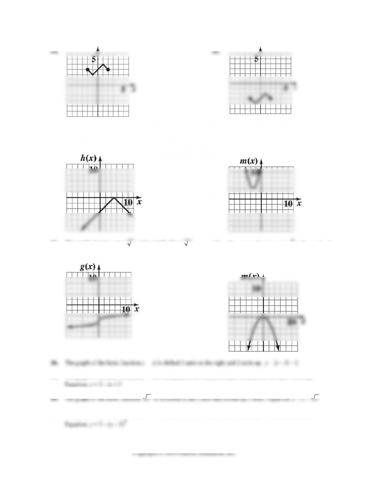
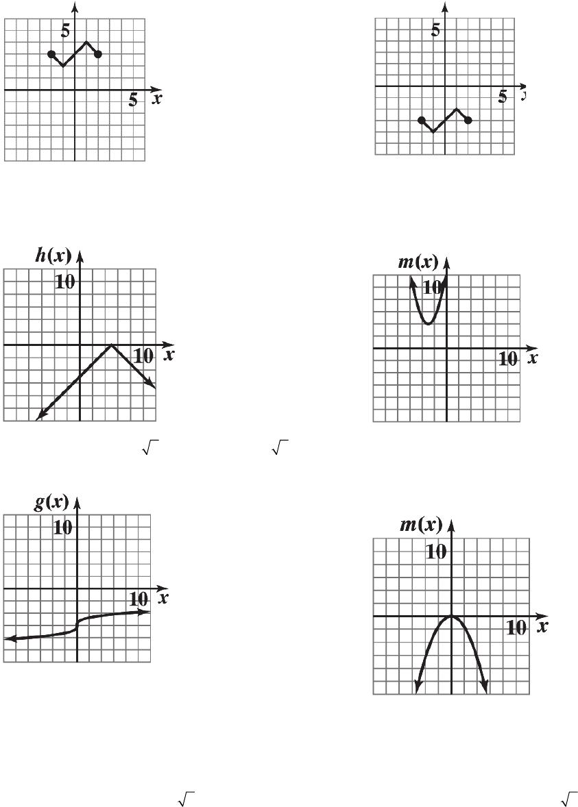
28. The graph of h(x) = –|x – 5| is the graph of y = |x|
reflected in the x axis and shifted 5 units to the right.
3
0. The graph of m(x) = (x + 3)2 + 4 is the graph of
y = x2 shifted 3 units to the left and 4 units up.
32. The graph of g(x) = –6 + 3
x
is the graph of y = 3
x
shifted 6 units down.
3
4. The graph of m(x) = –0.4x2 is the graph of
y = x2 reflected in the x axis and vertically
contracted by a factor of 0.4.
38. The graph of the basic function y = |x| is reflected in the x axis, shifted 2 units to the left and 3 units up.
x
x
42. The graph of the basic function y = x3 is reflected in the x axis, shifted to the right 3 units and up 1 unit.
EXERCISE 2-2 2-7
44. g(x) = 33x+ 2
46. g(x) = –|x – 1|
48. g(x) = 4 – (x + 2)2
50. 1if 1
()
22if 1
xx
gx xx
52. 10 2 if 0 20
() 40 0.5 if 20
xx
hx xx
54.
420if0 20
() 2 60 if 20 100
360 if 100
xx
hx x x
xx
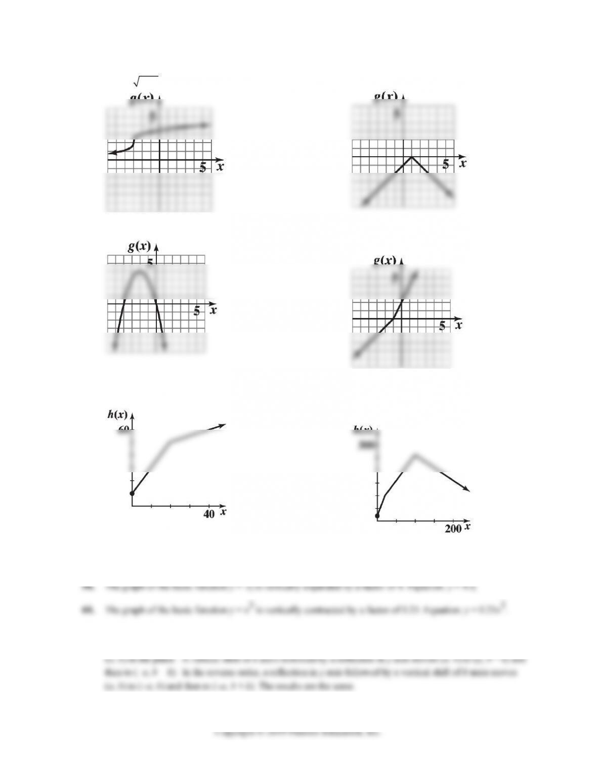
56. The graph of the basic function y = x is reflected in the x axis and vertically expanded by a factor of 2.
Equation: y = –2x
62. Vertical shift, reflection in y axis.
Reversing the order does not change the result. Consider a point
64. Vertical shift, vertical expansion.
Reversing the order can change the result. For example, let (a, b) be a point in the plane. A vertical shift of
66. Horizontal shift, vertical contraction.
Reversing the order does not change the result. Consider a point (a, b) in the plane. A horizontal shift of k
68. (A) The graph of the basic function y =
x
is
70. (A) The graph of the basic function y = x2 is
(B)
(B)
72. (A) Let x = number of kwh used in a winter
month. For 0 ≤ x ≤ 700, the charge is
8.5 .065 if 0 700
()
xx
Wx xx
(B)
74. (A) Let x = taxable income.
If 0 ≤ x ≤ 12,500, the tax due is $.02x. At x = 12,500, the tax due is $250. For 12,500 < x ≤ 50,000, the tax
0.02 if 0 12,500
0.06 1, 250 if 50,000
xx
xx
EXERCISE 2-3 2-9
(B)
(C) T(32,000) = $1,030
76. (A) The graph of the basic function y = x3 is
78. (A) The graph of the basic function y = 3
x
(B)
(B)
EXERCISE 2-3
2. 216
x
x (standard form) 4. 212 8xx (standard form)
264 6416xx (completing the square) 2
(8)64x (vertex form) 2
(1236)836xx
(6)44x (vertex form)
6. 2
31821xx (standard form)
2
3( 6 ) 21
xx
8. 2
51511xx (standard form)
2
5( ) 11
3
x
x
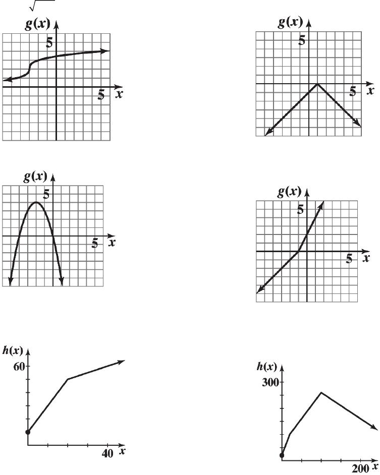
14. (A) g (B) m (C) n (D) f
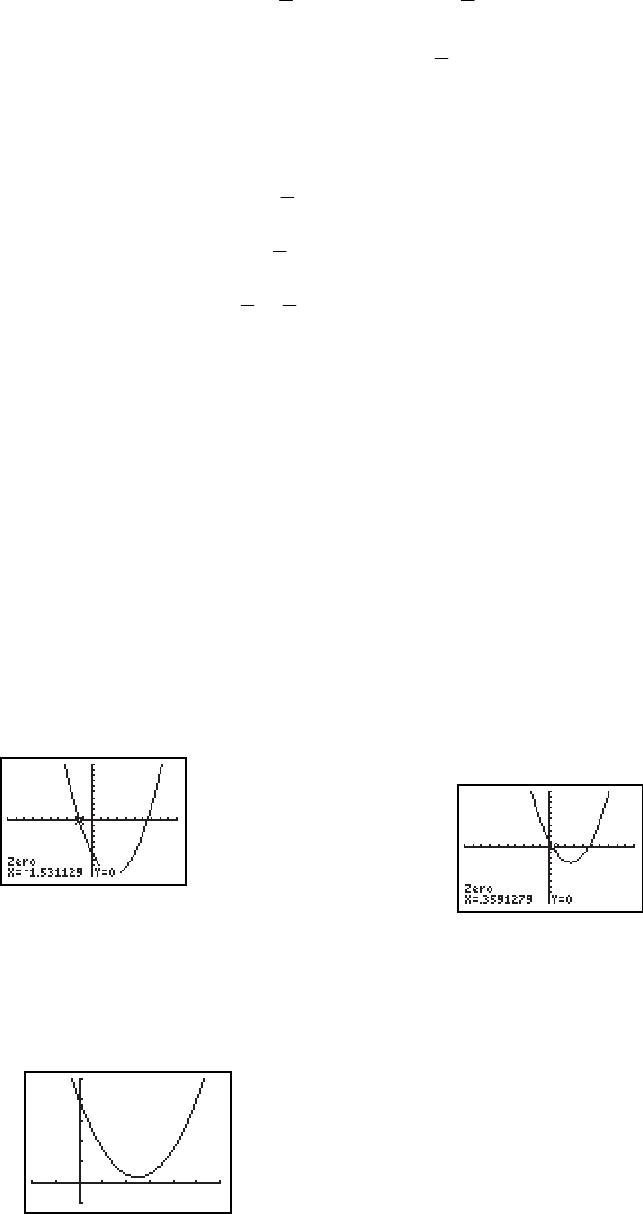
18. (A) x intercepts: 1, 5; y intercept: 5 (B) Vertex: (3, –4)
20. g(x) = –(x + 2)2 + 3
(A) x intercepts: –(x + 2)2 + 3 = 0
22. n(x) = (x – 4)2 – 3
(A) x intercepts: (x – 4)2 – 3 = 0
24. y = –(x – 4)2 + 2
26. y = [x – (–3)]2 + 1 or y = (x + 3)2 + 1
28. g(x) = x2 – 6x + 5 = x2 – 6x + 9 – 4 = (x – 3)2 – 4
(B) Vertex: (3, –4) (C) Minimum: –4 (D) Range: y ≥ –4 or [–4, ∞)
EXERCISE 2-3 2-11
30. s(x) = –4x2 – 8x – 3 = –4 23
24
xx
= –4 21
21
4
xx
= –4 21
(1)4
x
= –4(x + 1)2 + 1
(A) x intercepts: –4(x + 1)2 + 1 = 0
4(x + 1)2 = 1
32. v(x) = 0.5x2 + 4x + 10 = 0.5[x2 + 8x + 20] = 0.5[x2 + 8x + 16 + 4]
(A) x intercepts: none
34. g(x) = –0.6x2 + 3x + 4
(A) g(x) = –2: –0.6x2 + 3x + 4 = –2
0.6x2 – 3x – 6 = 0
(B) g(x) = 5: –0.6x2 + 3x + 4 = 5
–0.6x2 + 3x – 1 = 0
x = 0.36, 4.64
(C) g(x) = 8: –0.6x2 + 3x + 4 = 8
36. Using a graphing utility with y = 100x – 7x2 – 10 and the calculus option with maximum command, we
38. m(x) = 0.20x2 – 1.6x – 1 = 0.20(x2 – 8x – 5)
= 0.20[(x – 4)2 – 21] = 0.20(x – 4)2 – 4.2
(A) x intercepts: 0.20(x – 4)2 – 4.2 = 0
40. n(x) = –0.15x2 – 0.90x + 3.3 = –0.15(x2 + 6x – 22) = –0.15[(x + 3)2 – 31] = –0.15(x + 3)2 + 4.65
(A) x intercepts: –0.15(x + 3)2 + 4.65 = 0
42. (6)(3)0xx
44. 2712(3)(4)0xx x x
46.
48.
50.
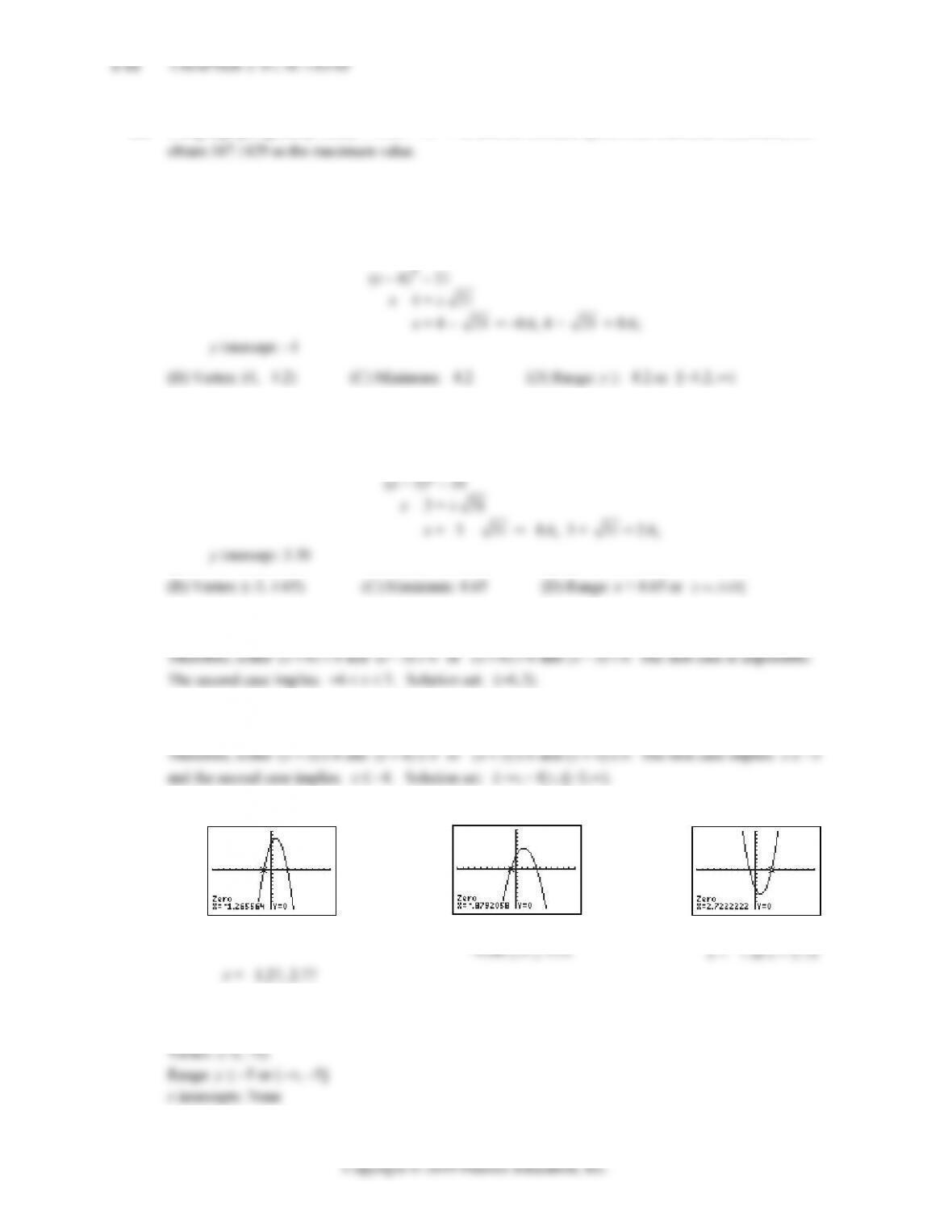
52. f is a quadratic function and max f(x) = f(–3) = –5
Axis: x = –3
54. (A)
(B) f(x) = g(x): –0.7x(x – 7) = 0.5x + 3.5
56. (A)
(B) f(x) = g(x): –0.7x2 + 6.3x = 1.1x + 4.8
–0.7x2 + 5.2x – 4.8 = 0
(C) f(x) > g(x) for 1.08 < x < 6.35
64. 22
22
()
(2 )
ax bx c a x h k
ax hx h k
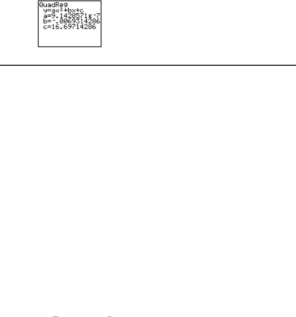
66. f(x) = –0.0117x2 + 0.32x + 17.9
(A)
Mkt Share ( )
5 18.8 19.2
15 20.7 20.1
25 17.4 18.6
35 15.3 14.8
x
fx
(B)
68. Verify
70. (A)
(B) R(x) = 2,000x – 60x2
= 2100
60 3
x
x
16.667 thousand computers
72. (A)
(B) R(x) = C(x)
x(2,000 – 60x) = 4,000 + 500x
(C) Loss: 1 ≤ x < 3.035 or 21.965 < x ≤ 25;
74. (A) P(x) = R(x) – C(x)
(B) and (C) Intercepts and break-even points: 3,035
76. Solve: f(x) = 1,000(0.04 – x2) = 30
40 – 1000x2 = 30
x = 0.10 cm
40
0
78.
For x = 2,300, the estimated fuel consumption is
EXERCISE 2-4
2. 2
() 56fx x
x
(2)(3)30
2, 3
xx
x
4. () 30 3
f
xx
(A) Degree: 1
10
x
6. 648
() 5 10fx x xx
(A) Degree: 8
8. 22
() ( 5)( 7)fx x x
(A) Degree: 4
10. 242
() (2 5)( 9)fx x x
(B)
(2 5) 9 0xx
12. (A) Minimum degree: 2
14. (A) Minimum degree: 3
16. (A) Minimum degree: 4
18. (A) Minimum degree: 5
20. A polynomial of degree 7 can have at most 7 x intercepts.
24. (A) Intercepts:
(B) Domain: all real numbers except x = –3
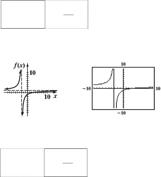
(C) Vertical asymptote at x = –3 by case 1 of the vertical asymptote procedure on page 57.
(D) (E)
26. (A) Intercepts:
x-intercept(s):
y-intercept:
x-intercept(s):
20
x
y-intercept:
2(0)
(0) 0
f
2-18 CHAPTER 2: FUNCTIONS
28. (A) Intercepts:
(B) Domain: all real numbers except 2x
(C) Vertical asymptote at x = 2 by case 1 of the vertical asymptote procedure on page 57.
3
0. (A)
x-intercept:
33 0
x
y-intercept:
33(0) 3
(B)
32. (A)
(B)
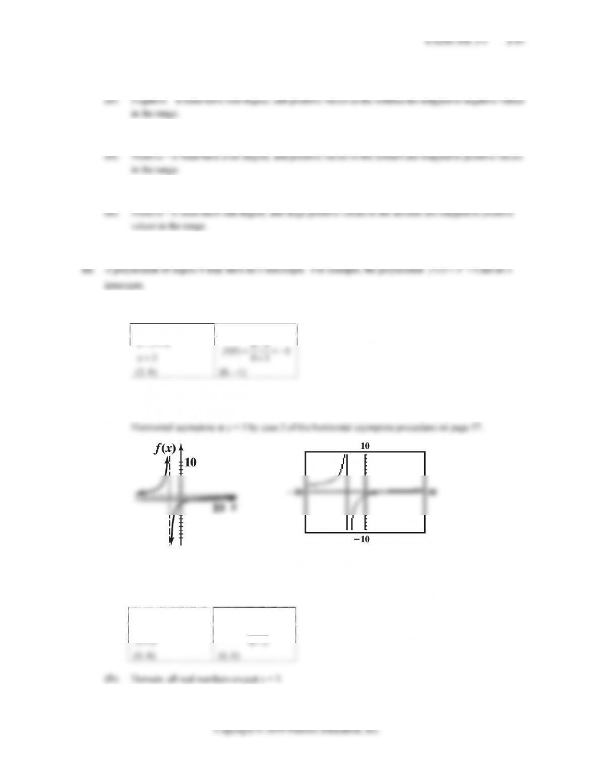
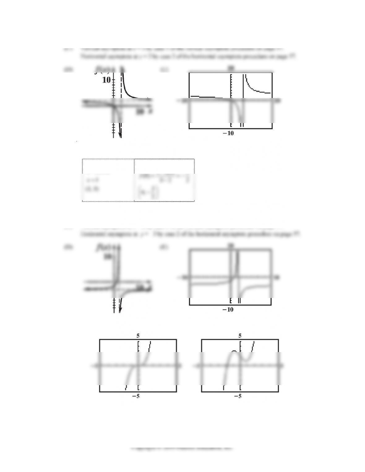
40. No horizontal asymptote, by case 3 for horizontal asymptotes on page 57.
42. Here we have denominator 22
( 4)( 16) ( 2)( 2)( 4)( 4)x x xxxx. Since none of these linear terms
44. Here we have denominator 278(1)(8)xx xx . Also, we have numerator
46. Here we have denominator 32 2
32 (32)(2)(1)xxxxxx xx x . We also have numerator
2-20 CHAPTER 2: FUNCTIONS
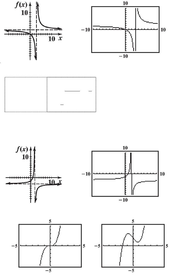
48. (A) Intercepts:
(B) Vertical asymptote when 26( 2)( 3)0xx x x ; so, vertical asymptotes at x = 2, x = –3.
Horizontal asymptote 3y.
(C) (D)
50. (A) Intercepts:
(B) Vertical asymptotes when 240x; i.e. at x = 2 and x = –2.
(C) (D)
52. (A) Intercepts:
30
0
x
x
x-intercept(s):
2
33 0
x
y-intercept:
3
(0) 4
f
x-intercept(s):
y-intercept: