EXERCISE 2-4 2-21
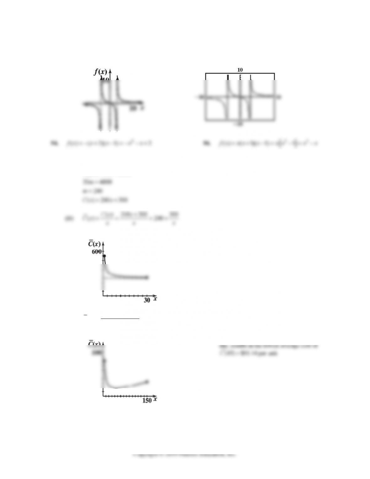
(B) Vertical asymptote when 212 ( 4)( 3) 0xx x x ; i.e. when x = – 4 and when x = 3.
Horizontal asymptote at y = 0.
(C) (D)
23
58. (A) We want ()Cx mx b. Fix costs are $300bper day. Given (20) 5,100Cwe have
(20) 300 5,100
m
x
xx
(C) (D) Average cost tends towards $240 as
production increases.
60. (A)
222,000
() xx
Cx x
(B) (C) A daily production level of x = 45 units per
2-22 CHAPTER 2: FUNCTIONS
(D)
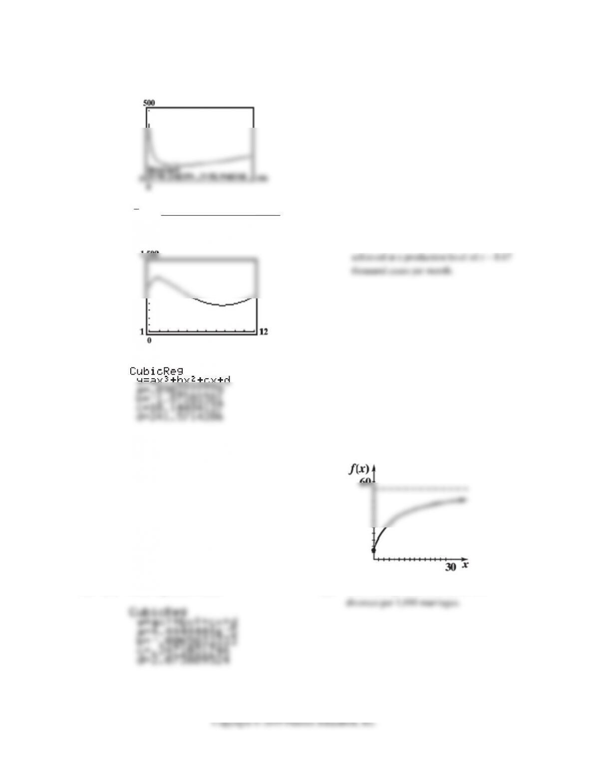
62. (A)
32
20 360 2,300 1,000
() xx x
Cx x
(B)
(C) A minimum average cost of $566.84 is
64. (A) Cubic regression model (B) (21) 583y eggs
66. (A) The horizontal asymptote is y = 55. (B)
68. (A) Cubic regression model (B) This model gives an estimate of 2.5
EXERCISE 2-5 2-23
Copyright © 2019 Pearson Education, Inc.
EXERCISE 2-5
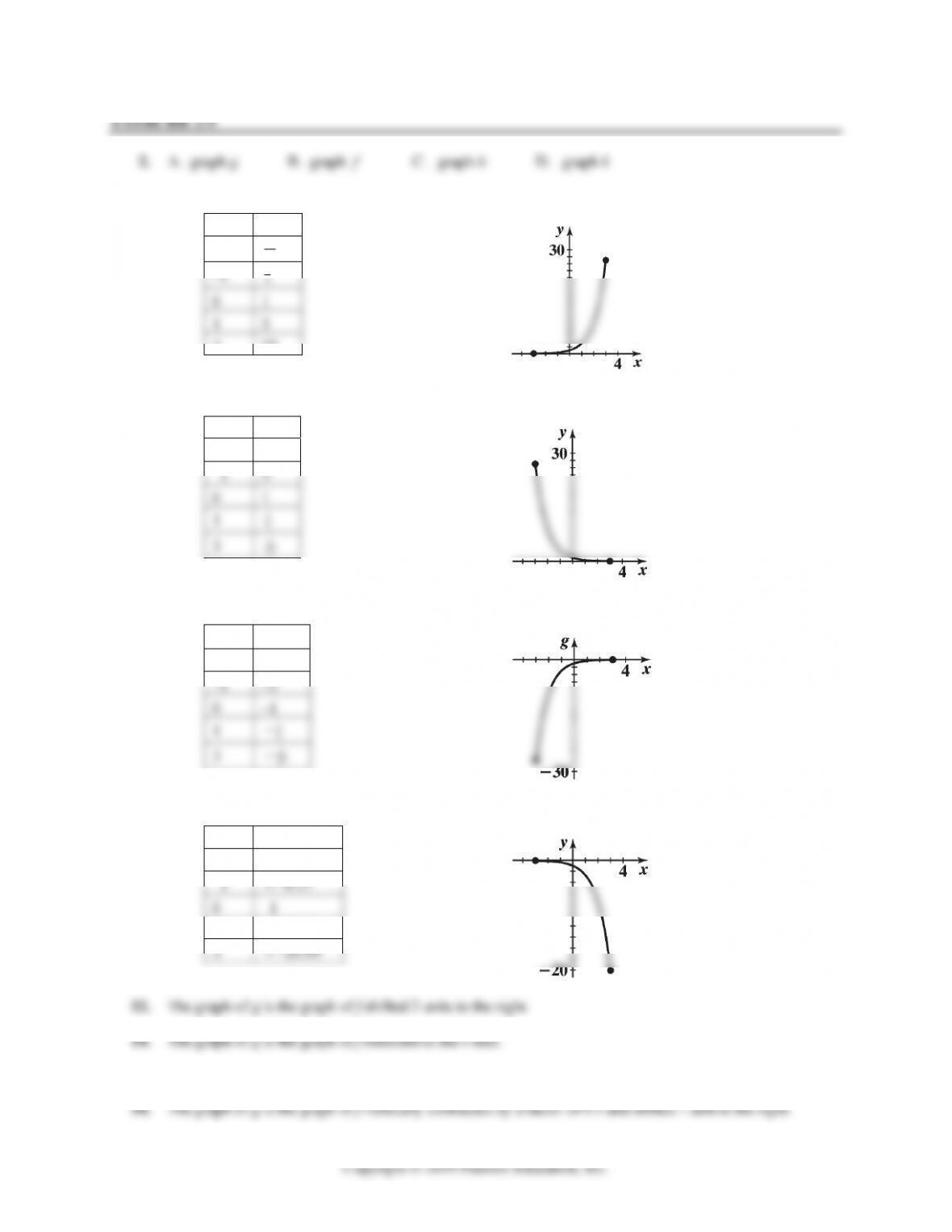
2. A. graph g B. graph f C. graph h D. graph k
4. 3;[ 3,3]
x
y
x
y
–3 1
27
3 27
6. 3;[3,3]
x
y
x
y
–
3 27
–
1 3
0 1
1 1
3
3 1
27
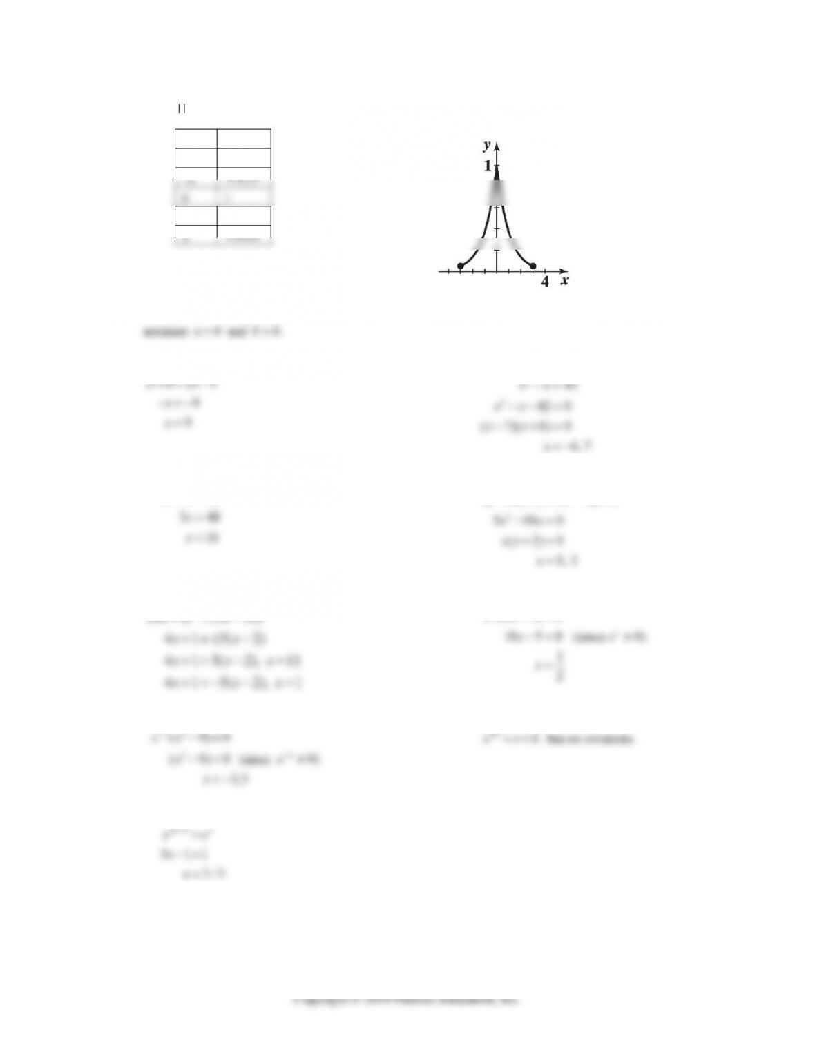
8. () 3 ;[3,3]
x
gx
x ()
g
x
–
3
–
27
–
1
–
3
–
27
10. ; [ 3, 3]
x
ye
x
y
–
3 0.05
–
–
1 2.72
16. The graph of g is the graph of f shifted 2 units down.
2-24 CHAPTER 2: FUNCTIONS
20. (A) () 2yfx
(B) (3)yfx
(C) 2() 4yfx
(D) 4(2)yfx
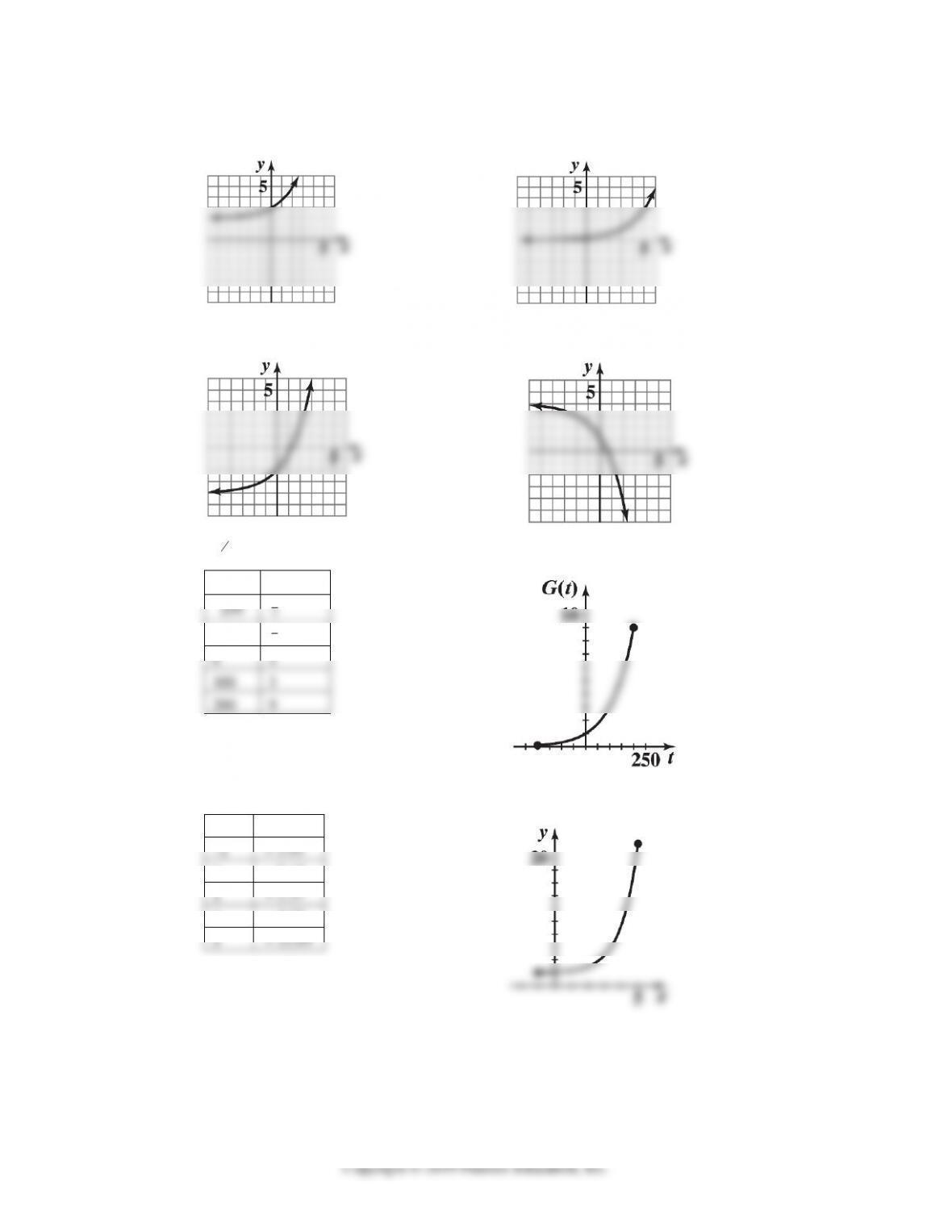
22. 100
( ) 3 ; [ 200, 200]
t
Gt
x ()Gt
–100 1
3
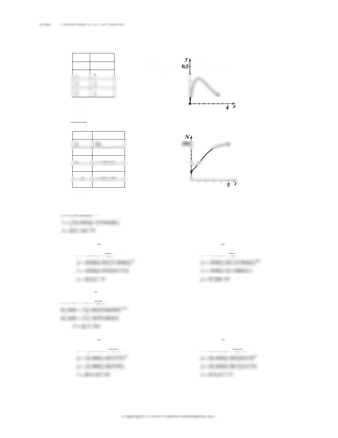
24. 2
2;[1,5]
x
ye
x
y
–
1 2.05
0 2.14
3 4.72
EXERCISE 2-5 2-25
26. ;[ 3,3]
x
ye
x
y
–
3 0.05
–
1 0.37
0 1
1 0.37
28. 2,a 2b for example. The exponential function property: For 0,x
x
x
ab if and only if ab
30. 425
33
xx
32. 242
2
55
xx
34. 44
(3 4) (52)
3452
x
x
36. 22
22
(2 1) (3 1)
441961
xx
x
xxx
38. 44
22
(4 1) (5 10)
xx
40. 10 5 0
xx
x
xe e
42. 2
90
xx
xe e
44. 4
0 for all ;
x
ee x
46. 31
0
x
ee
EXERCISE 2-6 2-27
(C)
(365)(5)
0.0125
(1 )
10,000(1 )
mt
r
m
AP
A
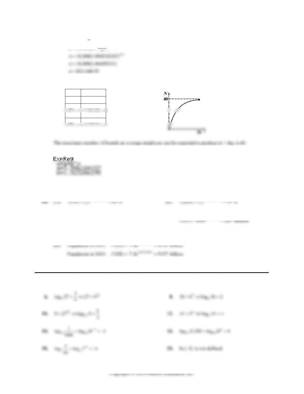
60. 0.12
40(1 ); [0, 30]
t
Ne
x
N
0 0
20 36.37
62. The exponential regression model (B) (10) 268.8y exabytes per month
o
o
66. (A) 0.0077
204 .
t
Pe (B) Population in 2030:
68. (A) 0.0113
7.4 t
Pe
EXERCISE 2-6
2. 5
2
log 32 5 32 2 4. 0
log 1 0 1
ee
3
22
64
2-28 CHAPTER 2: FUNCTIONS
22. 1
ln ( ) 1e 24. log log log
bbb
F
GFG
log log
PP
30. 10
log 1
x
32.
1
log 2
b
34. 49
log 7
y
36.
log 10, 000 2
b
38.
8
5
log 3
x
40. False; an example of a polynomial function of odd degree that is not one–to–one is 3
() .
f
xxx
42. False; the graph of every function (not necessarily one–to–one) intersects each vertical line at most once.
46. True; since g is the inverse of f, then (a, b) is on the graph of f if and only if (b, a) is on the graph of g.
48.
2
log log 27 2 log 2 log 3
3
bb bb
x
50.
1
log 3log 2 log 25 log 20
2
bb bb
x
EXERCISE 2-6 2-29
52.
2
log ( 2) log log 24
log ( 2) log 24
(6)(4)0
bbb
bb
xx
xx
xx
54. 10 10
log ( 6) log ( 3) 1
6
log 1
xx
x
56. 3
log ( 2)
32
32
y
y
yx
x
x
x
y
53
3
58. The graph of 3
log ( 2)yxis the graph of 3
logyx shifted to the left 2 units.
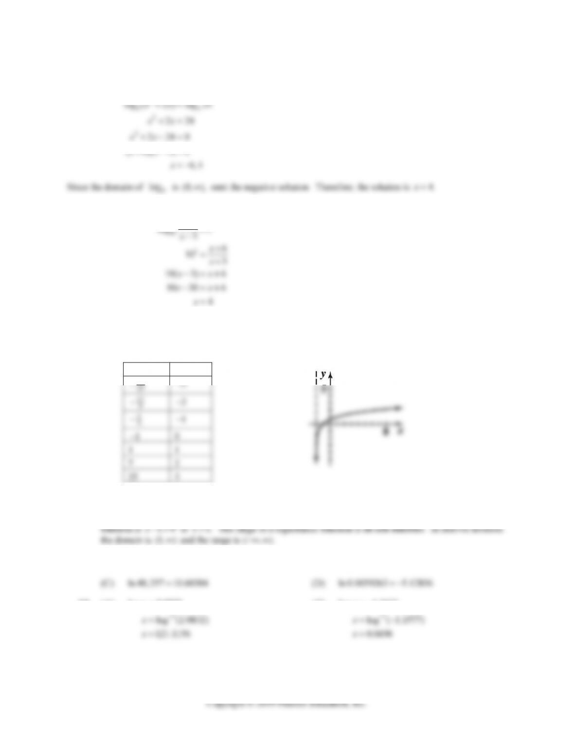
60. The domain of logarithmic function is defined for positive values only. Therefore, the domain of the
62. (A) log 72.604 1.86096 (B) log 0.033041 1.48095
64. (A)
log 2.0832
x
(B)
log 1.1577
x
2-32 CHAPTER 2: FUNCTIONS
Copyright © 2019 Pearson Education, Inc.
mt
r
m
(A) 2
0.08
2
2
7500 5000(1 )
1.5 (1.04)
t
t
(B) 12
0.08
12
12
7500 5000(1 )
1.5 (1.0066667)
t
t
88. Use the compound interest formula: .rt
A
Pe
0.0295
0.0295
41
17
41, 000 17,000
t
t
e
e
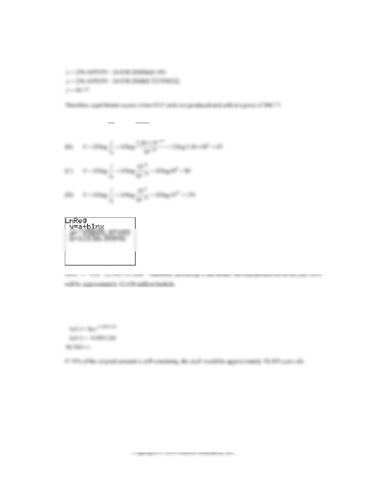
90. Equilibrium occurs when supply and demand are equal. The models from Problem 85 have the demand
and supply functions defined by 256.4659159 24.03812068lnyx and
127.8085281 20.01315349 ln , yxrespectively. Set both equations equal to each other to yield:
256.4659159 24.03812068ln 127.8085281 20.01315349ln
384.274444 44.05127417 ln
x
x
x
EXERCISE 2-6 2-33
Substitute the value above into either equation.
256.4659159 24.03812068 ln
yx
92. (A)
13 3
16
0
10
10log 10log 10log10 30
10
I
NI
10 6
3.16 10
I
16
0
10
94.
96. 0.000124
0
0.000124
00
0.000124
0.1
0.1
t
t
t
AAe
AAe
e
2-34 CHAPTER 2: FUNCTIONS
CHAPTER 2 REVIEW
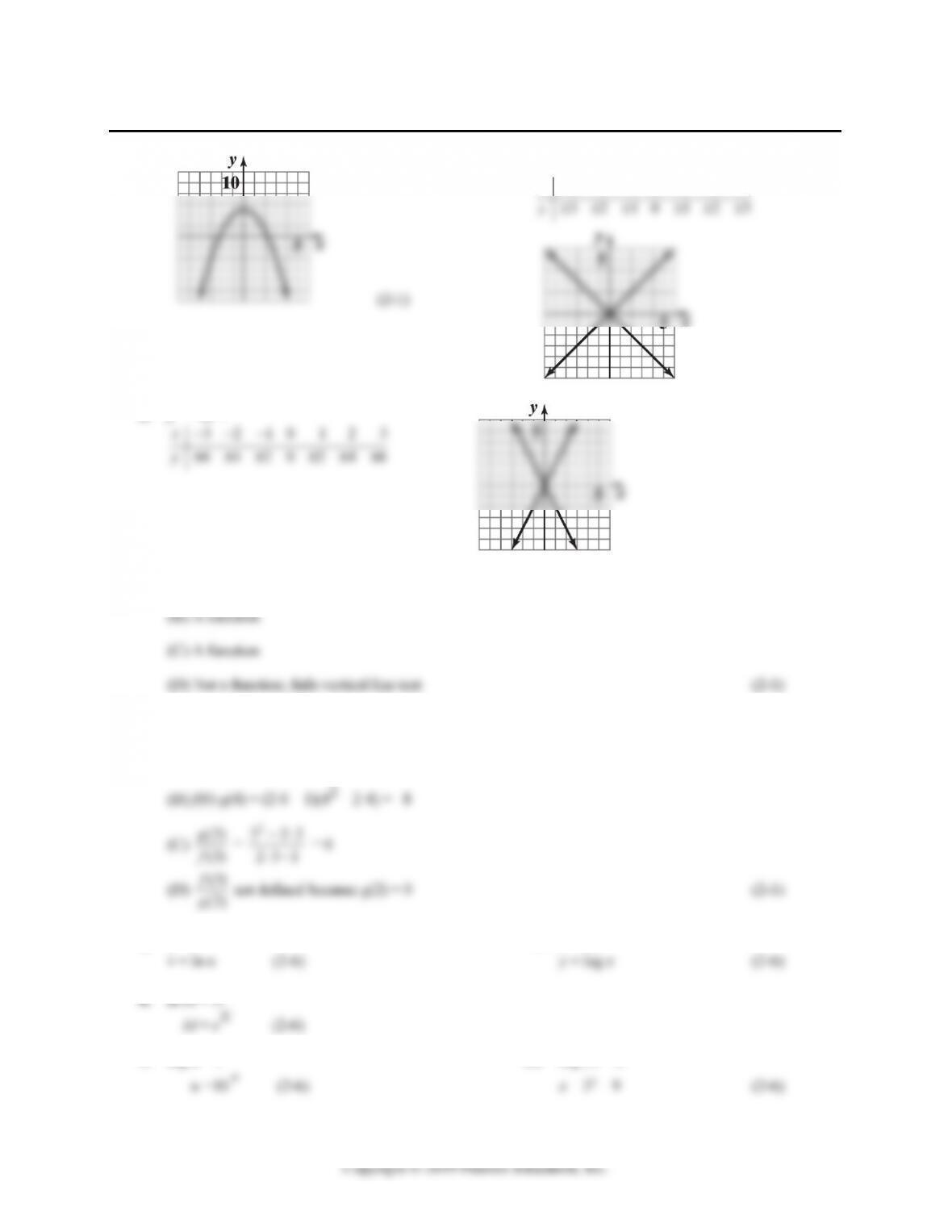
1.
2. x2 = y2:
3210123
x
(2-1)
3. y2 = 4x2:
6420246
y
(2-1)
4. (A) Not a function; fails vertical line test
5. f(x) = 2x – 1, g(x) = x2 – 2x
(A) f(–2) + g(–1) = 2(–2) – 1 + (–1)2 – 2(–1) = –2
6. u = ev 7. x = 10y
9. log u = v 10. log 3 x = 2