2 –
1
Chapter 2
Introduction to Probability
Learning Objectives
1. Obtain an understanding of the role probability information plays in the decision making process.
2. Understand probability as a numerical measure of the likelihood of occurrence.
5. Be able to use new information to revise initial (prior) probability estimates using Bayes’ theorem.
6. Know the definition of the following terms:
experiment addition law
sample space mutually exclusive
event conditional probability
Chapter 2
2 –
2
Solutions:
1. a. Go to the x-ray department at 9:00 a.m. and record the number of persons waiting.
b. The experimental outcomes (sample points) are the number of people waiting: 0, 1, 2, 3, and 4.
Note: While it is theoretically possible for more than 4 people to be waiting, we use what has
actually been observed to define the experimental outcomes.
Probability
0
.10
1
.25
2
.30
3
.20
4
.15
Total:
1.00
2. a. Choose a person at random, have her/ him taste the 4 blends and state a preference.
b. Assign a probability of 1/4 to each blend. We use the classical method of equally likely outcomes
here.
c.
Blend
Probability
1
.20
2
.30
3
.35
4
.15
Total:
1.00
The relative frequency method was used.
4. a. Of the 132,275,830 individual tax returns received by the IRS, 31,675,935were in the 1040A, Income
Under $25,000 category. Using the relative frequency approach, the probability a return from the 1040A,
Income Under $25,000 category would be chosen at random is 31675935/132275830 = 0.239.
b. Of the 132,275,830 individual tax returns received by the IRS, 3,376,943 were in the Schedule C,
Reciepts Under $25,000 category; 3,867,743 were in the Schedule C, Reciepts $25,000-$100,000
Introduction to Probability
2 –
3
c. Of the 132,275,830 individual tax returns received by the IRS, 12,893,802 were in the Non 1040A,
Income $100,000 & Over category; 2,288,550 were in the Schedule C, Reciepts $100,000 & Over
category; and 265,612 were in the Schedule F, Reciepts $100,000 & Over category. By the relative
frequency approach, the probability the chosen return reported income/reciepts of $100,000 and over is
(12893802 + 2288550 + 265612)/132275830 = 15447964/132275830 = 0.117.
5. a. No, the probabilities do not sum to one. They sum to 0.85.
b. Owner must revise the probabilities so that they sum to 1.00.
6. a. P(A) = P(150 – 199) + P(200 and over)
=
26 5
100 100
+
= 0.31
b. P(B) = P(less than 50) + P(50 – 99) + P(100 – 149)
= 0.13 + 0.22 + 0.34
= 0.69
8. a. Let P(A) be the probability a hospital had a daily inpatient volume of at least 200 and P(B) be the
probability a hospital had a nurse to patient ratio of at least 3.0. From the list of thirty hospitals, sixteen
had a daily inpatient volume of at least 200, so by the relative frequency approach the probability one of
these hospitals had a daily inpatient volume of at least 200 is P(A) = 16/30 = 0.533, Similarly, since ten
(one-third) of the hospitals had a nurse-to-patient ratio of at least 3.0, the probability of a hospital having
a nurse-to-patient ratio of at least 3.0 is P(B) = 10/30 = 0.333. Finally, since seven of the hospitals had
both a daily inpatient volume of at least 200 and a nurse-to-patient ratio of at least 3.0, the probability of a
hospital having both a daily inpatient volume of at least 200 and a nurse-to-patient ratio of at least 3.0
is P(A∩B) = 7/30 = 0.233.
Chapter 2
9. Let E = event patient treated experienced eye relief.
S = event patient treated had skin rash clear up.
Given:
P (E) = 90 / 250 = 0.36
P (S) = 135 / 250 = 0.54
P (E S) = 45 / 250 = 0.18
P (E S ) = P (E) + P (S) – P (E S)
= 0.36 + 0.54 – 0.18
= 0.72
11. a. Yes; the person cannot be in an automobile and a bus at the same time.
b. P(Bc) = 1 – P(B) = 1 – 0.35 = 0.65
12. a.
P(A B) 0.40
P(A B) 0.6667
P(B) 0.60
= = =
13. a.
Reason for Applying
Quality
Cost/Convenience
Other
Total
Full Time
0.218
0.204
0.039
0.461
Part Time
0.208
0.307
0.024
0.539
Total
0.426
0.511
0.063
1.00
b. It is most likely a student will cite cost or convenience as the first reason: probability = 0.511. School
quality is the first reason cited by the second largest number of students: probability = 0.426.
Introduction to Probability
2 –
5
e. P (B) = 0.426 and P (BA) = 0.473
Since P (B) P (BA), the events are dependent.
a. P(< 2 yrs) = .45
b. P(>= $1000) = .29
c. P(2 accounts have > = $1000) = (.29)(.29) = .0841
d. P($500-$999 | >= 2 yrs) = P($500-$999 and >= 2 yrs) / P(>=2yrs) = .275/.55 = .5
e. P(< 2 yrs and >=$1000) = .09
f. P(>=2 yrs | $500-$999) = .275/.515 = .533981
15. a. A joint probability table for these data looks like this:
Automobile Insurance Coverage
Yes No Total
For parts (b) through (g):
Let A= 18 to 34 age group
B= 35 and over age group
Y = Has automobile insurance coverage
N = Does not have automobile insurance coverage
b. We have P(A) = .46 and P(B) = .54, so of the population age 18 and over, 46% are ages 18 to 34 and 54%
are ages 35 and over.
Chapter 2
e. If the individual is age 35 or over, the probability the individual does not have automobile insurance
coverage is
( )
( )
( )
P.065
P B = = =.1204.
P .54
NB
NB
16. a. P(A B) = P(A)P(B) = (0.55)(0.35) = 0.19
b. P(A B) = P(A) + P(B) – P(A B) = 0.90 – 0.19 = 0.71
c. 1 – 0.71 = 0.29
17. a. P(attend multiple games) = 196 / 989 ≈ 19.8%.
b. P(male | attend multiple games) = 177 / 196 ≈ 90.3%.
c. P(male and attend multiple games) = P(male | attend multiple games) × P(attend multiple games) =
(177 / 196) × (196 / 989) = 177 / 989 ≈ 17.9%.
18. a. P(B) = 0.25
P(SB) = 0.40
P(S B) = 0.25(0.40) = 0.10
b.
P(S B) 0.10
P(B S) 0.25
P(S) 0.40
= = =
c. B and S are independent. The program appears to have no effect.
19. Let: A = lost time accident in current year
B = lost time accident previous year
Introduction to Probability
2 –
7
20. a. P(B A1) = P(A1)P(BA1) = (0.20)(0.50) = 0.10
b.
2
0.20
P(A B) 0.51
0.10 0.20 0.09
==
++
c.
Events
P(Ai)
P(BAi)
P(Ai B)
P(Ai B)
A1
0.20
0.50
0.10
0.26
A2
0.50
0.51
A3
0.30
0.30
0.09
0.23
21. S1 = successful, S2 = not successful and B = request received for additional information.
a. P(S1) = 0.50
22. a. Let F = female. Using past history as a guide, P(F) = .40
b. Let D = Dillard’s
.40(3/ 4) .30
P(F D) .67
.40(3/ 4) .60(1/ 4) .30 .15
= = =
++
The revised (posterior) probability that the visitor is female is .67.
We should display the offer that appeals to female visitors.
23. a. P(Oil) = 0.50 + 0.20 = 0.70
b. Let S = Soil test results
Events
P(Ai)
P(SAi)
P(Ai S)
P(Ai S)
High Quality (A1)
0.50
0.20
0.10
0.435
Medium Quality (A2)
0.20
0.174
No Oil (A3)
0.30
0.391
Chapter 2
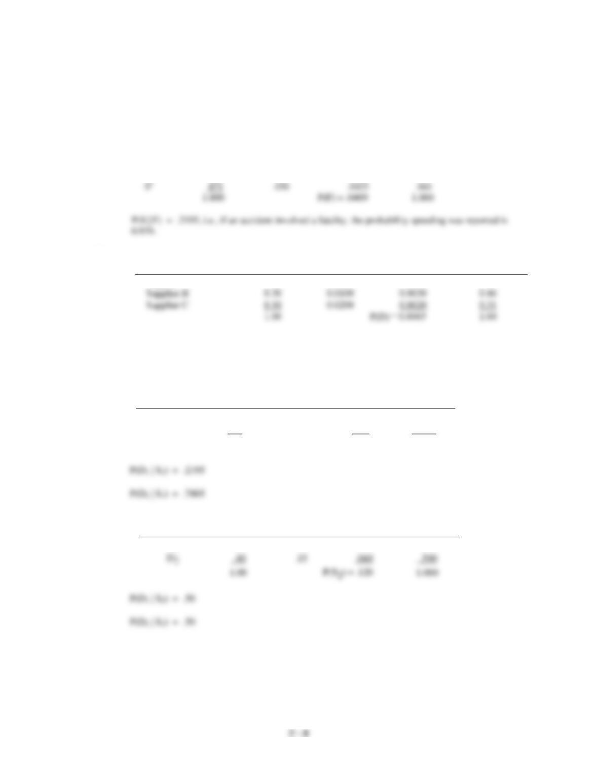
24. Let S= speeding is reported
SC= speeding is not reported
F = Accident results in fatality for vehicle occupant
We have P(S) = .129, so P(SC) = .871. Also P(F|S) = .196 and P(F|SC) = .05. Using the tabular form
of Bayes’ Theorem provides:
Prior Conditional Joint Posterior
Events Probabilities Probabilities Probabilities Probabilities
S .129 .196 .0384 .939
25.
Events
P(Ai)
P(DAi)
P(AiD)
P(AiD)
Supplier A
0.60
0.0025
0.0015
0.23
Supplier B
0.30
0.0100
0.0030
0.46
Supplier C
0.10
0.0200
0.0020
0.31
a. P(D) = 0.0065
b. B is the most likely supplier if a defect is found.
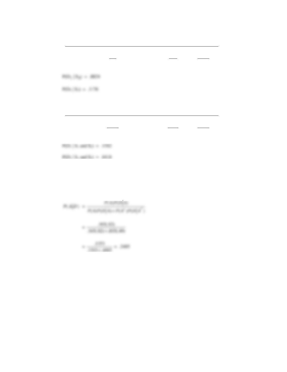
26. a.
Events
P(Di)
P(S1|Di)
P(Di S1)
P(Di |S1)
D1
.60
.15
.090
.2195
D2
.40
.80
.320
.7805
1.00
P(S1) = .410
1.0000
b.
Events
P(Di)
P(S2 |Di)
P(Di S2)
P(Di |S2)
D1
.60
.10
.060
.500
D2
.40
.15
.060
1.00
P(S2) = .120
Introduction to Probability
2 –
9
c.
Events
P(Di)
P(S3 |Di)
P(Di S3)
P(Di |S3)
D1
.60
.15
.090
.8824
D2
.40
.03
.012
.1176
1.00
P(S3) = .102
1.0000
d. Use the posterior probabilities from part (a) as the prior probabilities here.
Events
P(Di)
P(S2 | Di)
P(Di S2)
P(Di | S2)
D1
.2195
.10
.0220
.1582
D2
.7805
.15
.1171
.8418
1.0000
.1391
1.0000
27. a. Let A = age 65 or older
( ) 1 .835 .165PA= − =
b. Let D = takes drugs regularly
28. a. P(A1) = .095
P(A2) = .905
P(W | A1) = .60
P(W | A2) = .49
Chapter 2
2 –
10
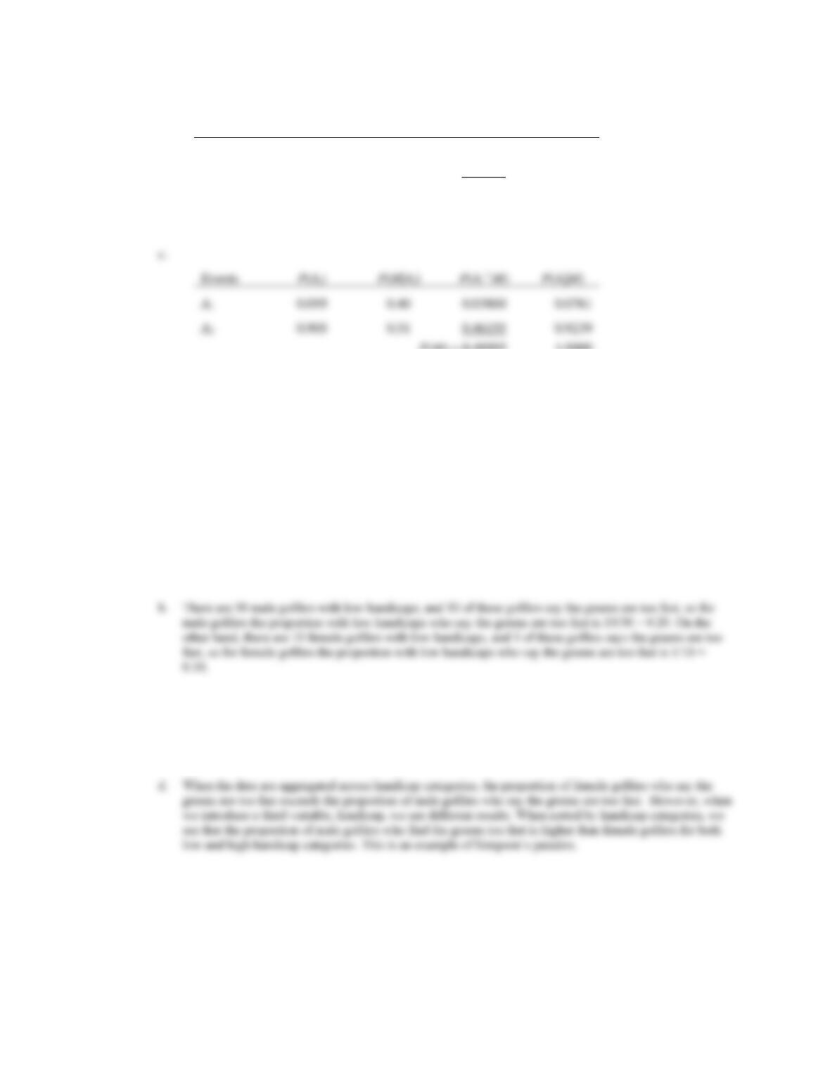
b.
Events
P(Ai)
P(W|Ai)
P(Ai∩W)
P(Ai|W)
A1
0.095
0.60
0.05700
0.1139
A2
0.905
0.49
0.44345
0.8861
P(W) = 0.50045
1.0000
P(A1|W) = .1139
Events
P(Ai)
P(M|Ai)
P(Ai∩M)
P(Ai|M)
0.095
0.40
0.03800
0.0761
0.905
0.51
0.46155
0.9239
P(M) = 0.49995
1.0000
P(A1|M) = .0761
d. P(W) = .50045
P(M) = .49965
29. a.
Gender Too Fast Acceptable
Male Golfers 35 65
Female Golfers 40 60
The proportion of male golfers who say the greens are too fast is 35/(35 + 65) = 0.35, while the proportion
of female golfers who say the greens are too fast is 40/(40 + 60) = 0.40. There is a higher percentage of
female golfers who say the greens are too fast.
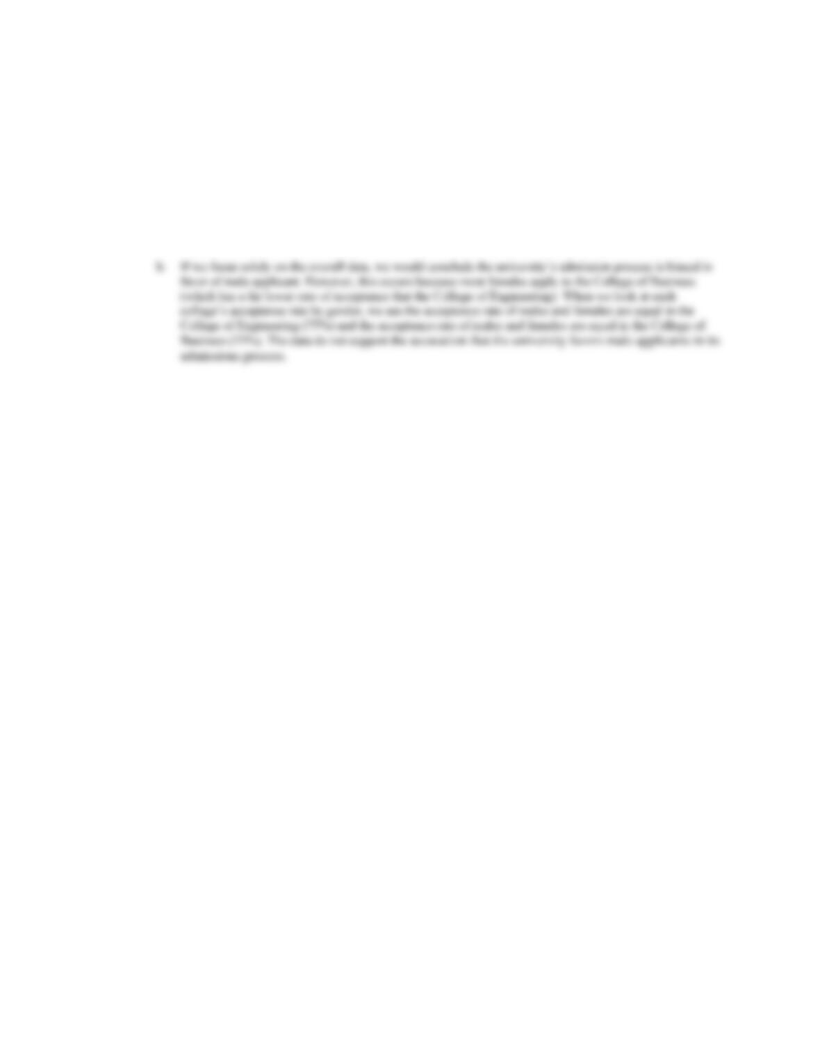
c. There are 50 male golfers with higher handicaps, and 25 of these golfers say the greens are too fast, so for
male golfers the proportion with higher handicaps who say the greens are too fast is 25/50 = 0.50. On the
other hand, there are 90 female golfers with higher handicaps, and 39 of these golfers says the greens are
too fast, so for female golfers the proportion with higher handicaps who say the greens are too fast is
39/90 = 0.43.
Introduction to Probability
2 –
11
30. a.
Male Applicants Female Applicants
Accept 70 40
Deny 90 80
After combining these two crosstabulations into a single crosstabulation with Accept and Deny as the row
labels and Male and Female as the column labels, we see that the rate of acceptance for males across the
university is 70/(70+90) = .4375 or approximately 44%, while the rate of acceptance for females across
the university is 40/(40+80) = .33 or 33%.