Chapter 19 – Linear Programming
19-1
CHAPTER 19
LINEAR PROGRAMMING
Teaching Notes
The main goal of this supplement is to provide the students with an overview of the types of problems
that have been solved using linear programming (LP). In the process of learning the different types of
problems that can be solved with LP, the students must also develop a very basic understanding of the
assumptions and special features of LP problems.
The students should also learn the basics of developing and formulating linear programming models
for simple problems, solve two-variable linear programming problems by the graphical procedure and
interpret the resulting outcome. In the process of solving these graphical problems, we must stress the
role and importance of extreme points in obtaining an optimal solution.
Answers to Discussion and Review Questions
1. Linear programming is well-suited to an environment of certainty.
2. The “area of feasibility,” or feasible solution space is the set of all combinations of values of
3. Redundant constraints do not affect the feasible region for a linear programming problem.
4. An iso-cost line represents the set of all possible combinations of two inputs that will result in
5. Sliding an objective function line towards the origin represents a decrease in its value (i.e.,
6. a. Basic variable: In a linear programming solution, it is a variable not required to equal
zero.
b. Shadow price: It is the change in the value of the objective function per unit increase in a
constraint right hand side.
Chapter 19 – Linear Programming
19-2
Solution to Problems
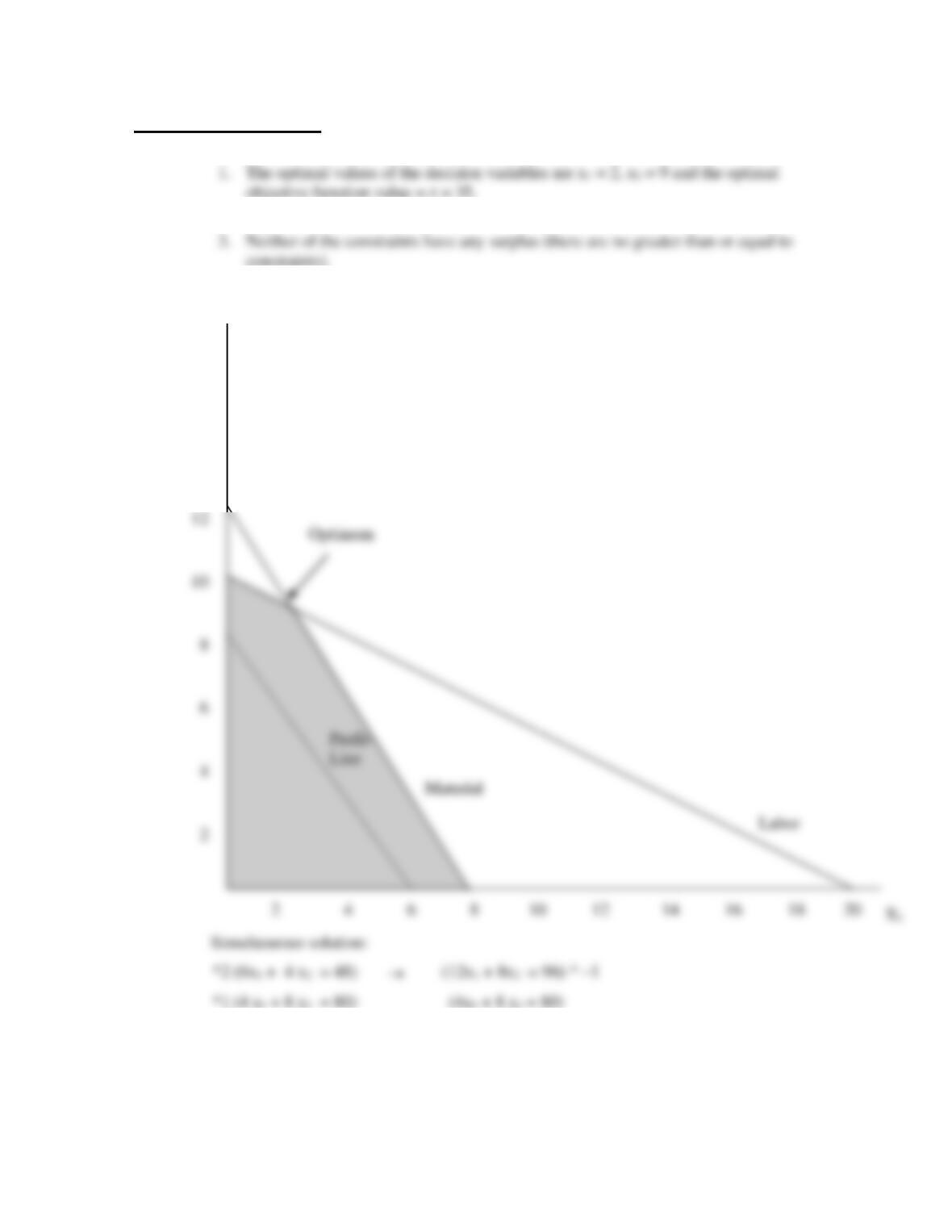
1. a.
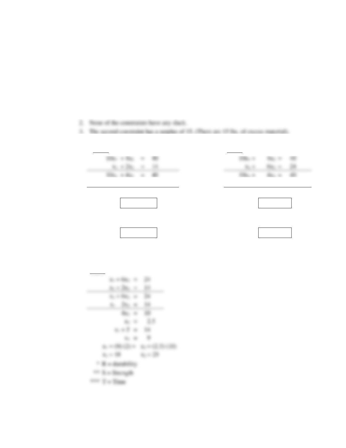
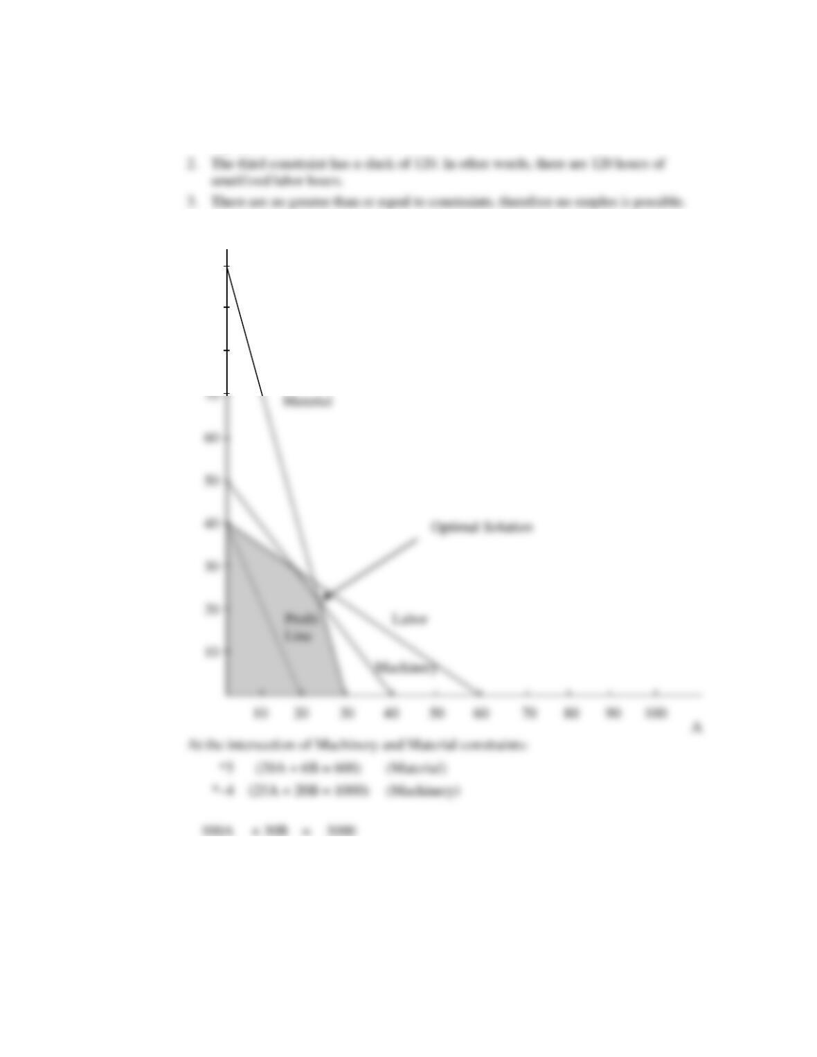
2. None of the constraints have any slack. Both constraints are binding.
4. No, there are no redundant constraints.
X2
18
16
14
Chapter 19 – Linear Programming
19-3
–12x1
– 8x2
= –96
4x1
+ 8x2
= 80
4x1
+ 8x2
= 80
4(2)
+ 8x2
= 80
–8x1
= –16
8x2
= 72
x1
= 2
x2
= 9
z = 4x1 + 3x2 = 4(2) + 3(9) = 35
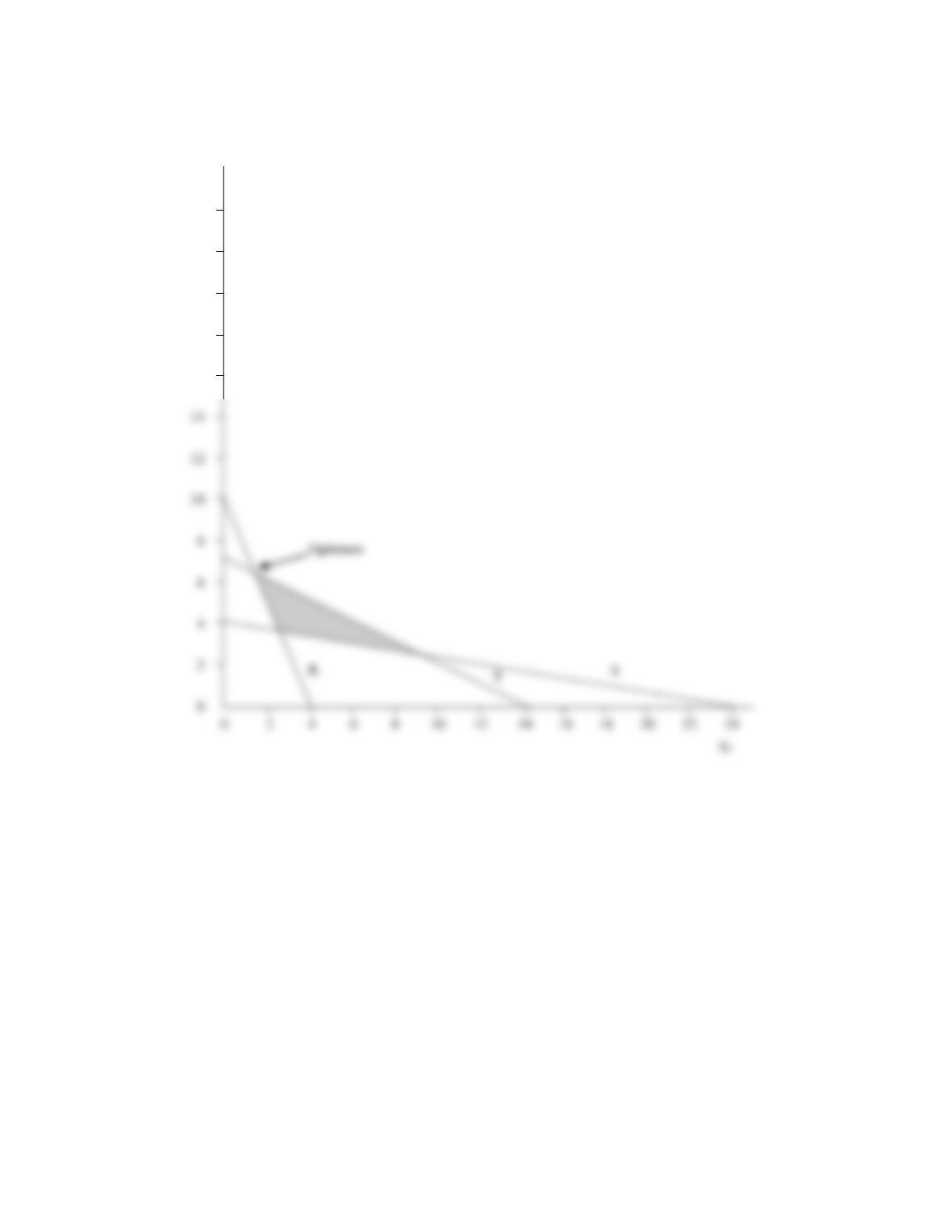
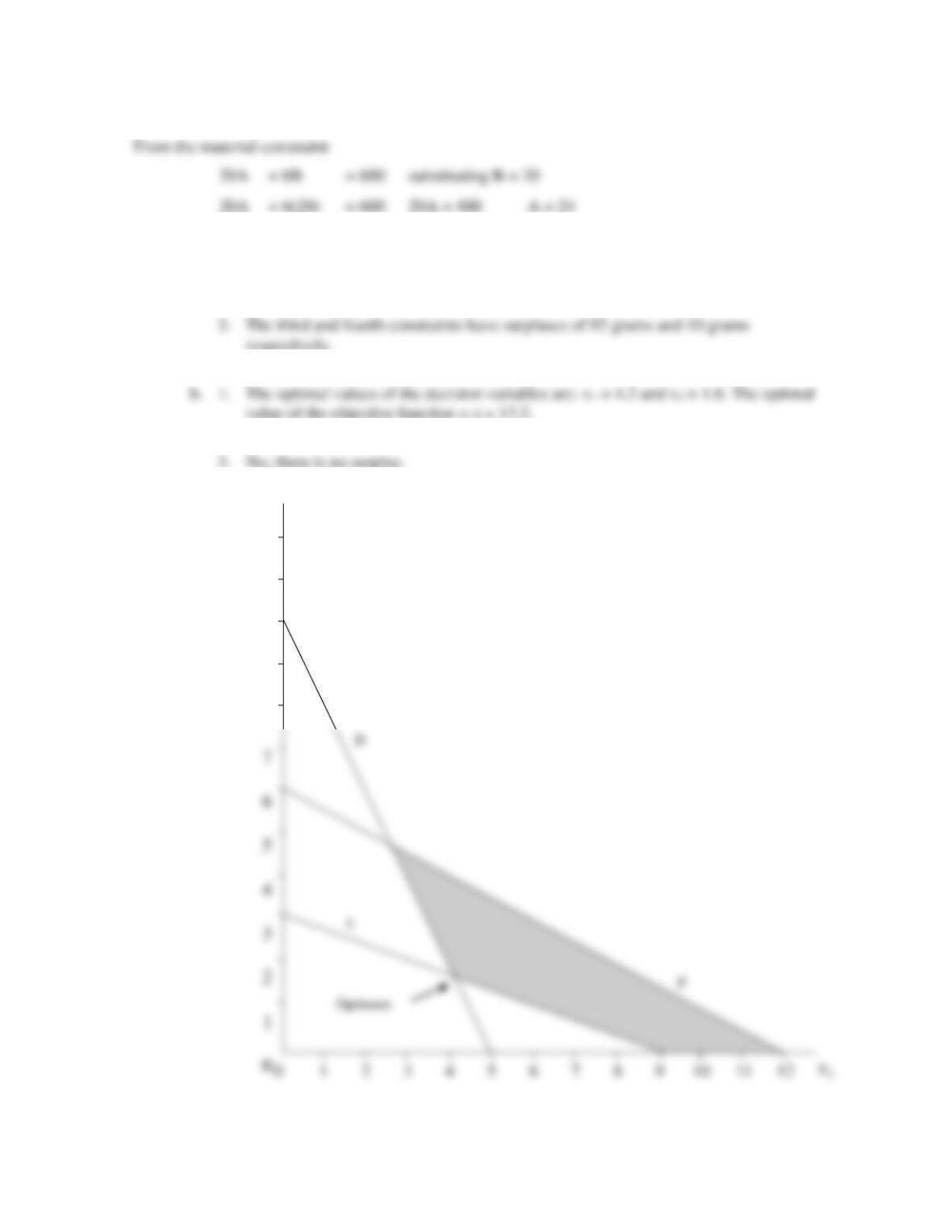
b. 1. The optimal values of the decision variables are x1 = 1.5, x2 = 6.25 and the optimal
objective function value z = 65.5.
4. No, there are no redundant constraints.
*R & T (Optimum)
R & S**
= 40
= 40
= 14
= 24
–2x1
– 4x2
= –28
–10x1 –
60x2
= –240
8x1
= 12
–
56x2
= –200
x1 = 1.5
x2 = 3.57
1.5 + 2x2
= 14
x1 + 21.42
= 24
2x2
= 12.5
x2 = 6.25
x1 = 2.58
x1 = (1.5) (2), x2 = (6.25) (10)
x1 = (2.58) (2), x2 = (3.57) (10)
x1 = 3, x2 = 62.5
x1 = 5.16, x2 = 35.7
x1 + x2 = 65.5
x1 + x2 = 40.86
S & T***
Chapter 19 – Linear Programming
19-4
X2
24
22
20
18
16
Chapter 19 – Linear Programming
19-5
c. 1. The optimal values of the decision variables are A = 24, B = 20 and the optimal
objective function value = z = 204.
4. No, there are no redundant constraints.
(25A + 20B = 1000)
(Machinery)
= 3000
Labor
Machinery
Material
–100A
– 80B
= –4000
–50B
= –1000
B
= 20
100
90
80
B
Chapter 19 – Linear Programming
19-6
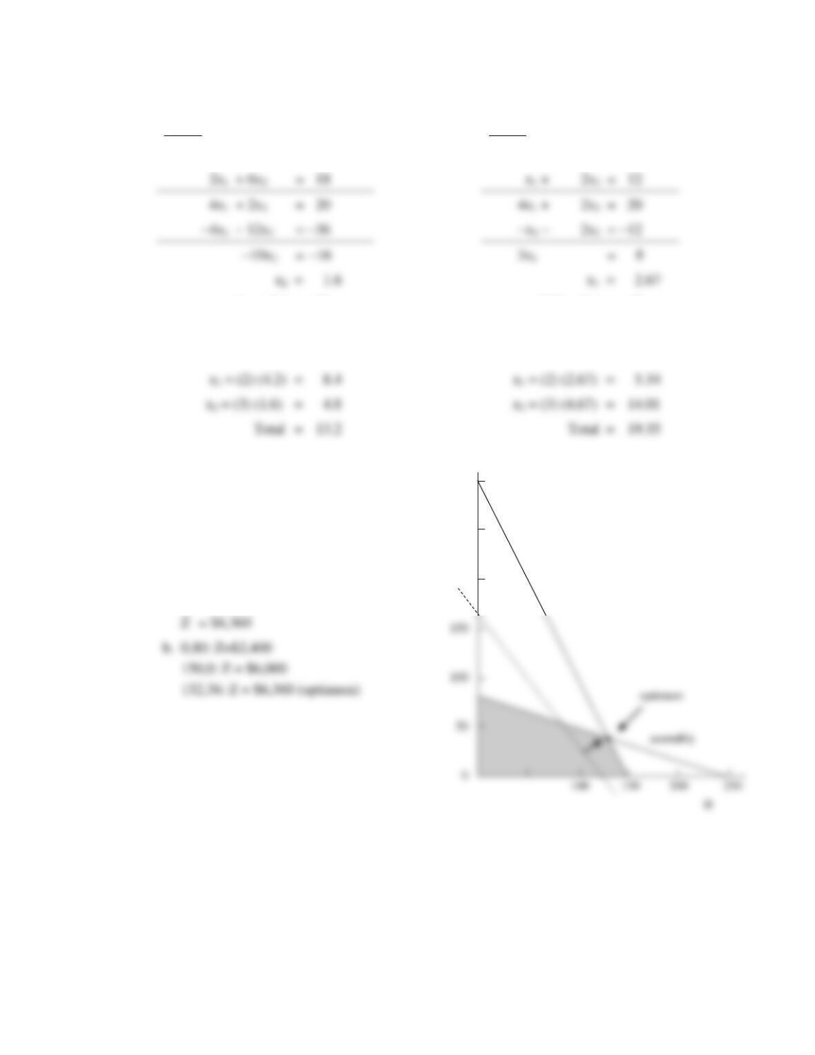
2. a. 1. The optimal values of the decision variables are: S = 8 and T = 20. The optimal
objective function value = z = 58.4.
2. Since all of the constraints are greater than or equal to type, none of the constraints
have any slack.
4. Yes, the third constraint is redundant. It does not affect the feasible region.
2. Yes, the constraint F has a slack of 4.6.
4. No, there are no redundant constraints.
12
11
10
9
8
X2
Chapter 19 – Linear Programming
19-7
Solutions (continued)
D & E
D & F
4x1
+ 2x2
= 20
4x1 +
2x2
= 20
4x1 + 3.2
= 20
2.67 + 2x2
= 12
4x1
= 16.8
2x2
= 9.33
x1
= 4.2
x2
= 4.67
x1 = (2) (2.67) = 5.34
x2 = (3) (4.67) = 14.01
Total = 19.35
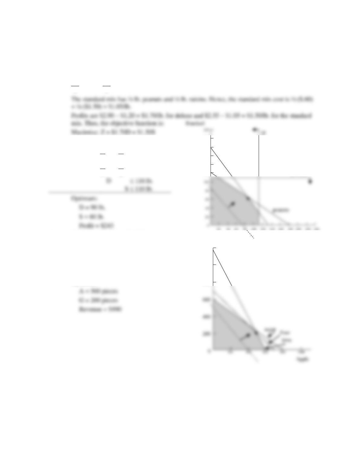
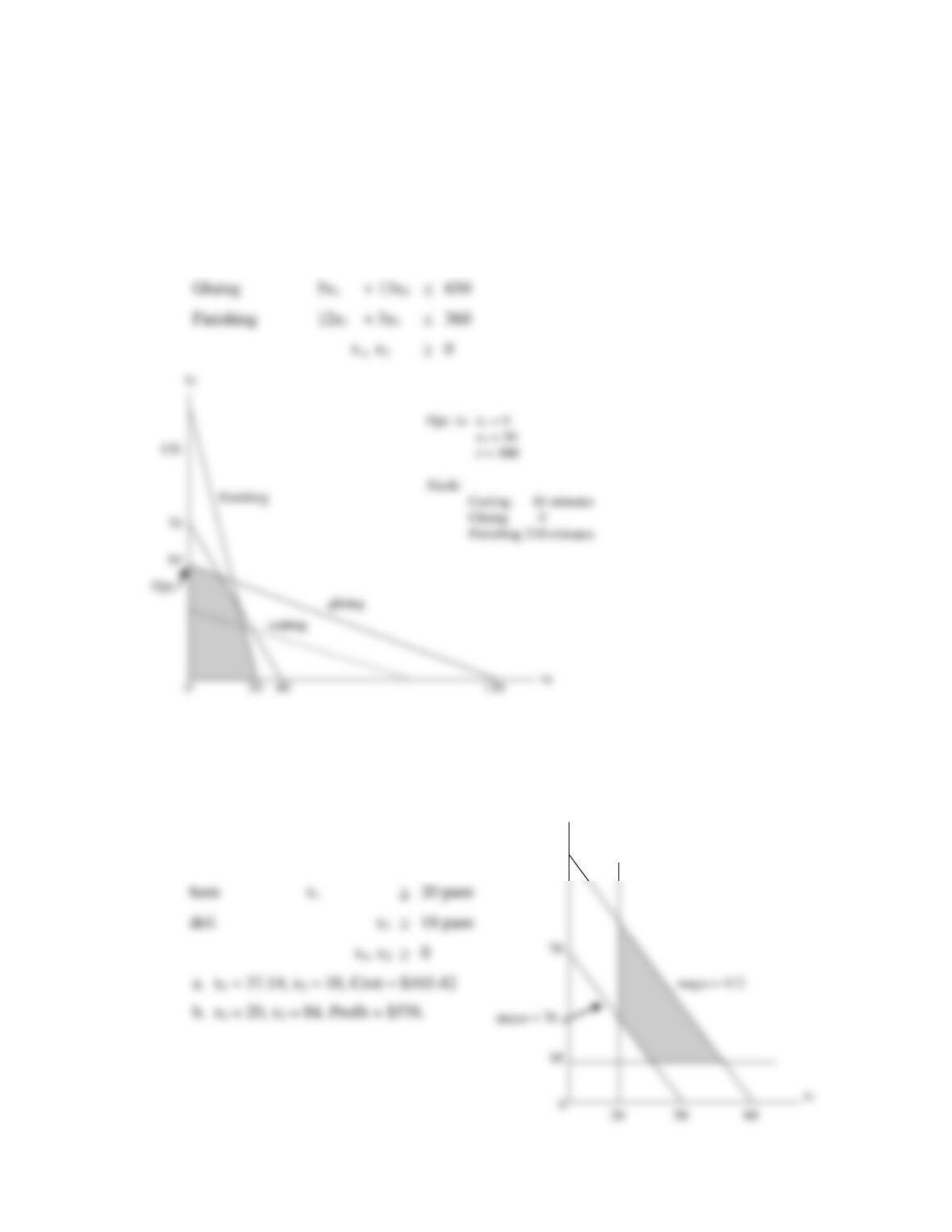
3. Maximize: $40H + $30W
Subject to:
fabrication 4H + 2W 600 hours
assembly 2H + 6W 480 hours
a. Optimum:
H = 132
W = 36
assembly
H
300
250
200
W
fabrication
= 18
= 12
+ 2x2
= 20
4x1 +
2x2
= 20
= –36
= –12
= –16
= 8
x2
= 1.6
x1
= 2.67
Chapter 19 – Linear Programming
19-8
Solutions (continued)
4. Peanuts cost $.60/lb. Deluxe revenue is $2.90/lb.
Raisins cost $1.50/lb. Standard revenue is $2.55 /lb.
Deluxe mix has 1/3 lb. peanuts, 2/3 lb. raisins. Hence, deluxe mix cost is
1
($.60) +
2
($1.50) = $1.20/lb.
3
3
Subject to:
raisins
2
D +
1
S 90 lb.
3
2
peanuts
1
D +
1
S 60 lb.
3
2
peanuts
5. Maximize: $1.50A + $1.20G
Subject to:
sugar: 1.5A + 2.0G 1,200 cups
flour: 3.0A + 3.0G 2,100 cups
time: 6.0A + 3.0G 3,600 min.
Optimum:
S = 110
Deluxe
raisins
200
180
160
140
120
Grape
1200
1000
800
Chapter 19 – Linear Programming
19-9
Solutions (continued)
Unused supplies
sugar: 1.5(500) + 2(200) = 1,150 cups used. Hence, 1,200 – 1,150 = 50 cups
remaining.
6. a. The optimal value of the decision variables are: x1 = 4, x2 = 0, x3 = 18. The optimal value
of the objective function value = z = 106.
b. The optimal value of the decision variables are: x1 = 15, x2 = 10, x3 = 0. The optimal
value of the objective function value = z = 210.
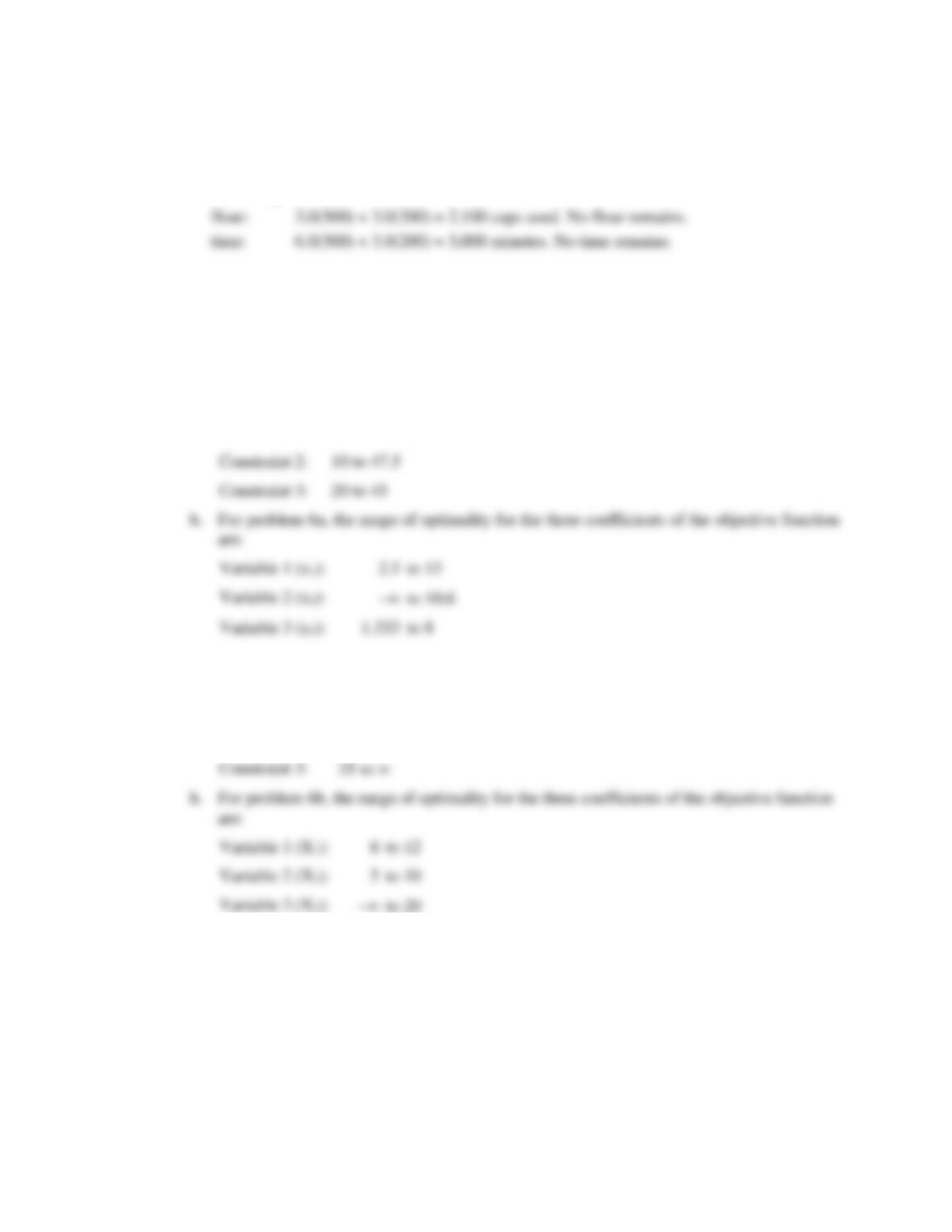
7. a. For problem 6a, the range of feasibility for the three constraints are as follows:
Constraint 1:
22 to infinity ()
Constraint 2:
10 to 47.5
Constraint 3:
20 to 45
Variable 1 (x1):
2.5 to 15
Variable 3 (x3):
1.333 to 8
8. a. For problem 6b, the range of feasibility for the three constraints are as follows:
Constraint 1:
20 to 26.6667
Constraint 2:
35 to 50
Constraint 3:
35 to
Variable 1 (X1):
6 to 12
Variable 2 (X2):
5 to 10
Chapter 19 – Linear Programming
19–10
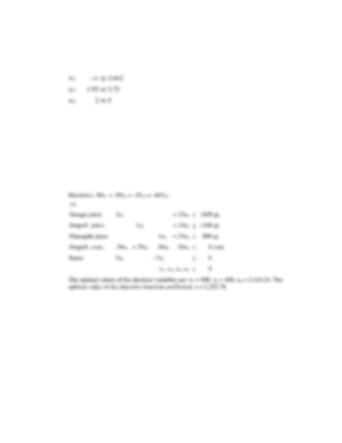
9. The optimal value of the decision variables are: x1 = 0, x2 = 80, x3 = 50. The optimal value of
the objective function is z = 350. The range of optimality for the profit coefficient of each
variable is as follows:
10. x1 = number of containers of orange juice
x2 = number of containers of grapefruit juice
x3 = number of containers of pineapple juice
x4 = number of containers of All-in-One
Orange Juice
Grapefruit Juice
Pineapple Juice
All-in-One
Revenue per qt.
$1.00
$.90
$.80
$1.10
Cost per qt.
.50
.40
.35
.417
Profit per qt.
$.50
$.50
$.45
$.683
Chapter 19 – Linear Programming
19–11
11. x1 = qty. of chopping boards
x2 = qty. of knife holders
maximize
2x1
+ 6x2
s.t.
Cutting
1.4x1
+ .8x2
56 minutes
12. x1 = qty. ham spread
x2 = qty. deli spread
maximize
2x1
+ 4x2
(profit) or minimize 3x1 + 3x2 (cost)
s.t.
mayo
1.4x1
+ 1.0x2
70 lb.
mayo
1.4x1
+ 1.0x2
112 lb.
0
x1 = 37.14, x2 = 18, Cost = $165.42
b.
x1 = 20, x2 = 84, Profit = $376.
x2
112
Finishing
12x1
+ 3x2
360
x2
0
Chapter 19 – Linear Programming
19–12
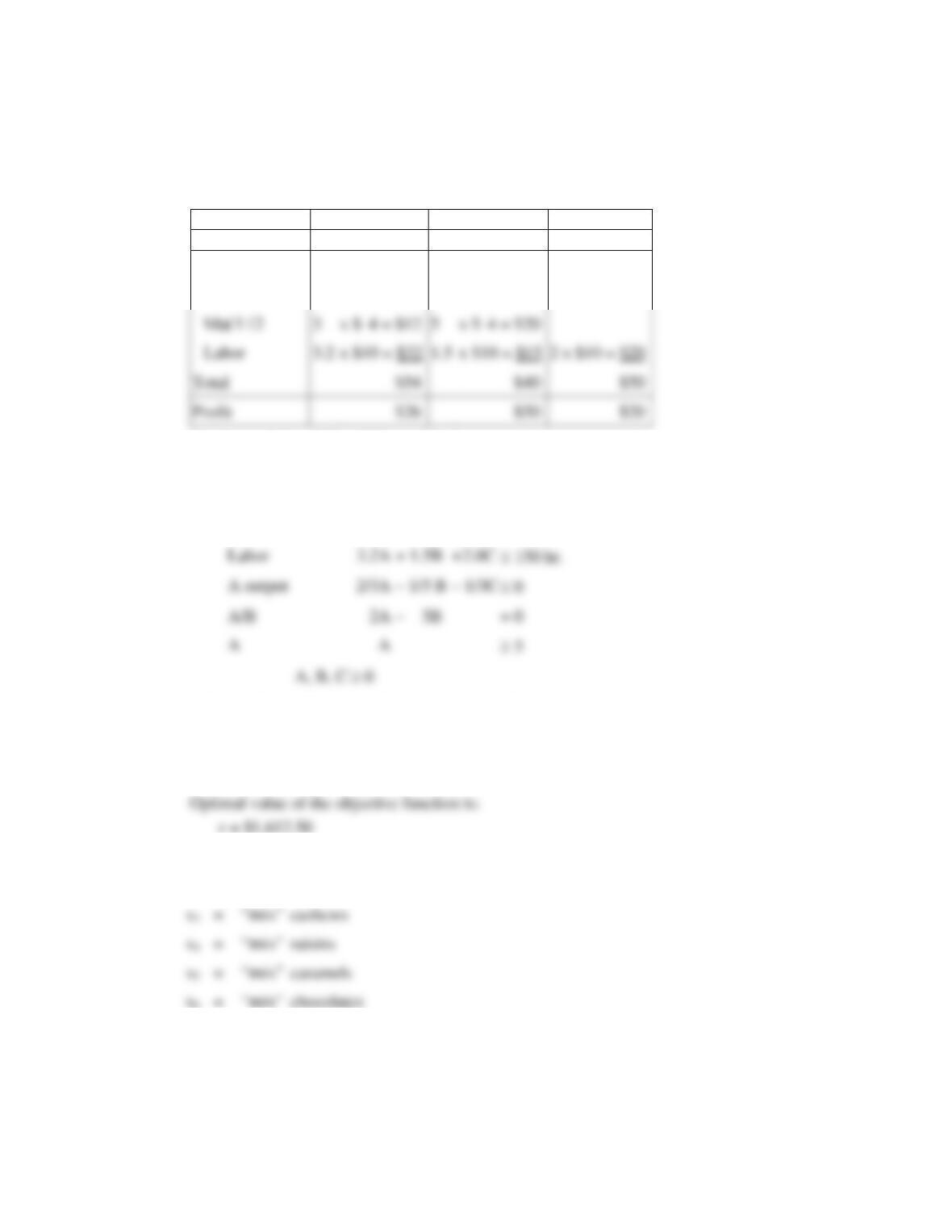
13. A = quantity of product A
B = quantity of product B
C = quantity of product C
A
B
C
Revenue
$80
$90
$70
Cost
Mat’l #1
2
x $ 5 = $10
1
x $ 5 = $ 5
6 x $ 5 = $30
Maximize 26A + 50B + 20C (profit)
s.t.
Mat’l #1
2A
+ 1B
+ 6C
200 lb.
Mat’l #2
3A
+ 5B
300 lb.
Labor
+ 1.5B
+ 2.0C
150 hr.
A/B
= 0
A
5
Solution: Optimal values of the decision variables are:
A = 18.75
B = 12.50
C = 25.00
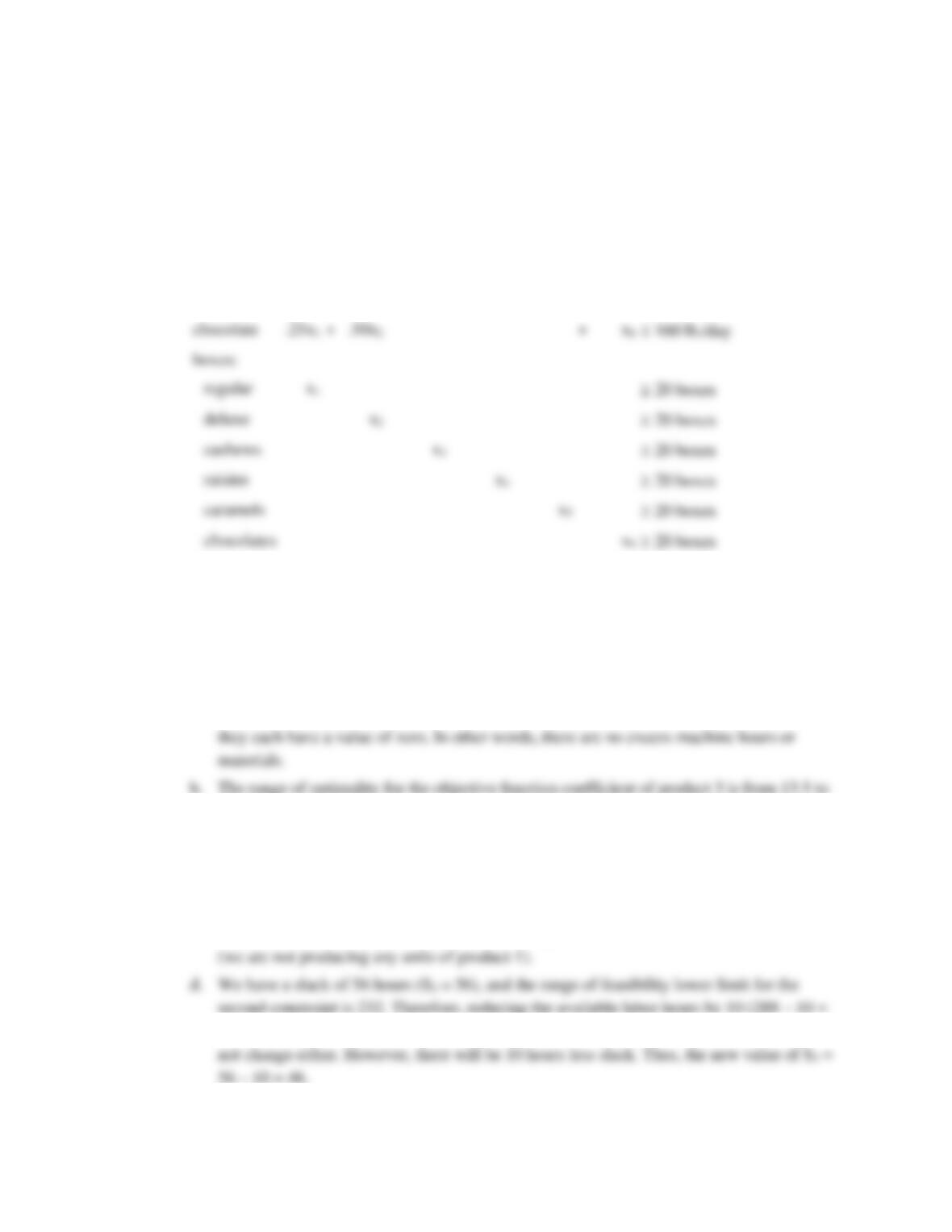
14.
x1
= boxes of regular mix
x2
=
“mix”
deluxe
x3
=
“mix”
cashews
x4
=
raisins
x5
=
“mix”
caramels
x6
=
chocolates
x $ 4 = $12
5
x $ 4 = $20
3.2
x $10 = $32
1.5
x $10 = $15
2 x $10 = $20
Total
$54
$40
$50
Profit
$26
$50
$20
Chapter 19 – Linear Programming
19–13
maximize
.80x1
+ .90x2
+ .70x3
+ .60x4
+ .50x5
+ .75x6
s.t.
cashews
.25x1
+ .50x2
+ x3
120 lb./day
raisins
.25x1
+ x4
200 lb./day
caramels
.25x1
+ x5
100 lb./day
x1, x2, x3, x4, x5, x6 0
Solution:
x1
= 320
x4
= 120
x2
= 40
x5
= 20
Z = 433
x3
= 20
x6
= 60
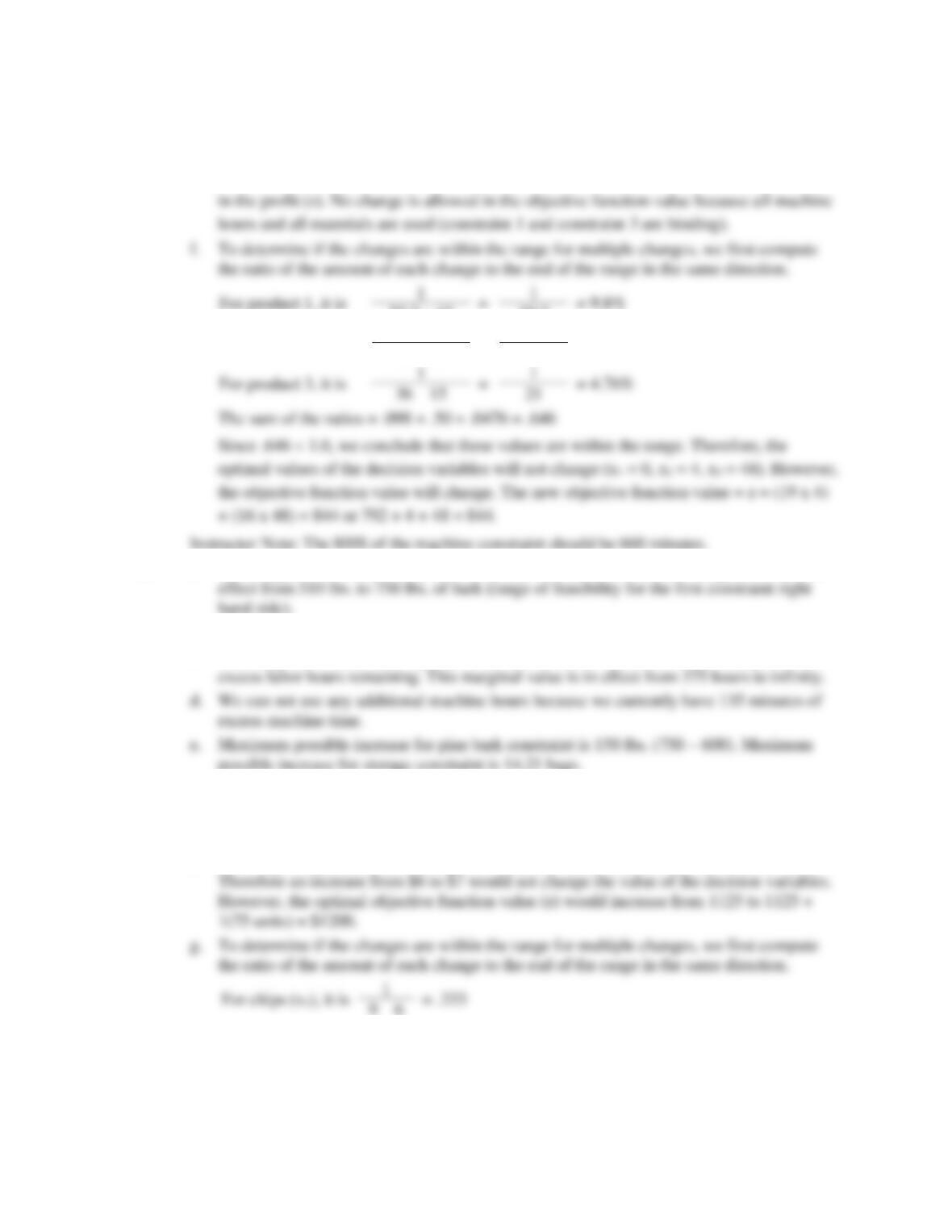
15. a. The first constraint (machine) and the third constraint (material) are binding because S1
and S3 are not in the solution (are not basic variables). Therefore as nonbasic variables,
36. Therefore an increase from 15 to 22 would not change the value of the decision
variables. However, the objective function value would increase from 792 to 792 + 48 (22
– 15). Therefore the new value of z = 1128.
c. The range of optimality for the objective function coefficient of product 1 is from – to
22.2. Since 22 is within the range, the change would not affect the value of decision
variables. Since x1 is not a basic variable, the objective function value will not be affected
278) will not affect the value of the decision variables. The objective function value will
chocolate
.25x1
+ .50x2
+ x6
160 lb./day
boxes:
20 boxes
20 boxes
20 boxes
20 boxes
20 boxes
20 boxes
Chapter 19 – Linear Programming
19–14
e. If no additional machine hours and materials are obtained, there would not be any change
22.2 – 12
10.2
For product 2, it is
1
=
1
= 50%
20 – 18
2
For product 3, it is
=
= 4.76%
36 – 15
16. a. The marginal value (shadow price) of a pound of bark is $1.50. This marginal value is in
b. 1.50 per pound.
c. The marginal value (shadow price) of 1 labor hour is zero because we currently have 105
(1.50) (150) = $225 (expected increase in profit for pine bark)
(1.50) (14.21) = $21.32 (expected increase in profit for storage)
Therefore, add 150 pounds of pine bark.
f. The range of optimality for the objective function coefficient of chips (x3) is from 5.4 to 9.
= .333
For product 1, it is
1
=
1
= 9.8%
Chapter 19 – Linear Programming
19–15
For nuggets (x1), it is
.6
= .600
9 – 8
h. To determine if the changes are within the range for multiple changes, we first compute
the ratio of the amount of each change to the end of the range in the same direction.
For pine barks (first constraint), it is
15
= .10
750 – 600
For machine time (second constraint), it is
27
= .36
600 – 525
= .352
164.21 – 150
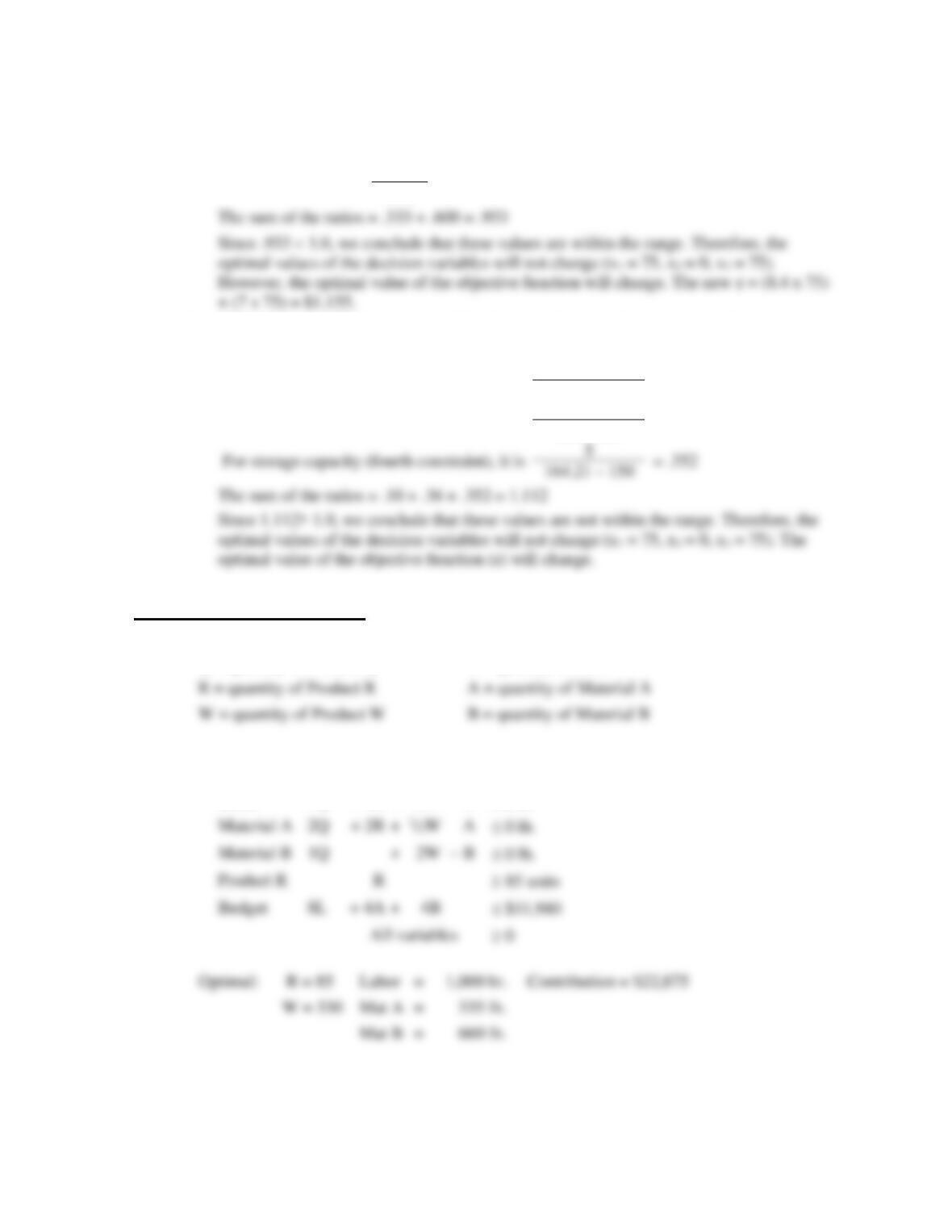
Solution to Son, Ltd. Case
Q = quantity of Product Q
L = quantity of labor
W = quantity of Product W
B = quantity of Material B
1. Maximize 122Q + 115R + 76W – 8L – 4A – 4B
subject to
Labor
5Q
+ 4R
+
2W
– L
0 hr.
Material B
1Q
+
0 lb.
Product R
85 units
0
Optimal:
R = 85
Labor =
Contribution = $22,875
W = 330
Mat A =
Mat B =
Chapter 19 – Linear Programming
19–16
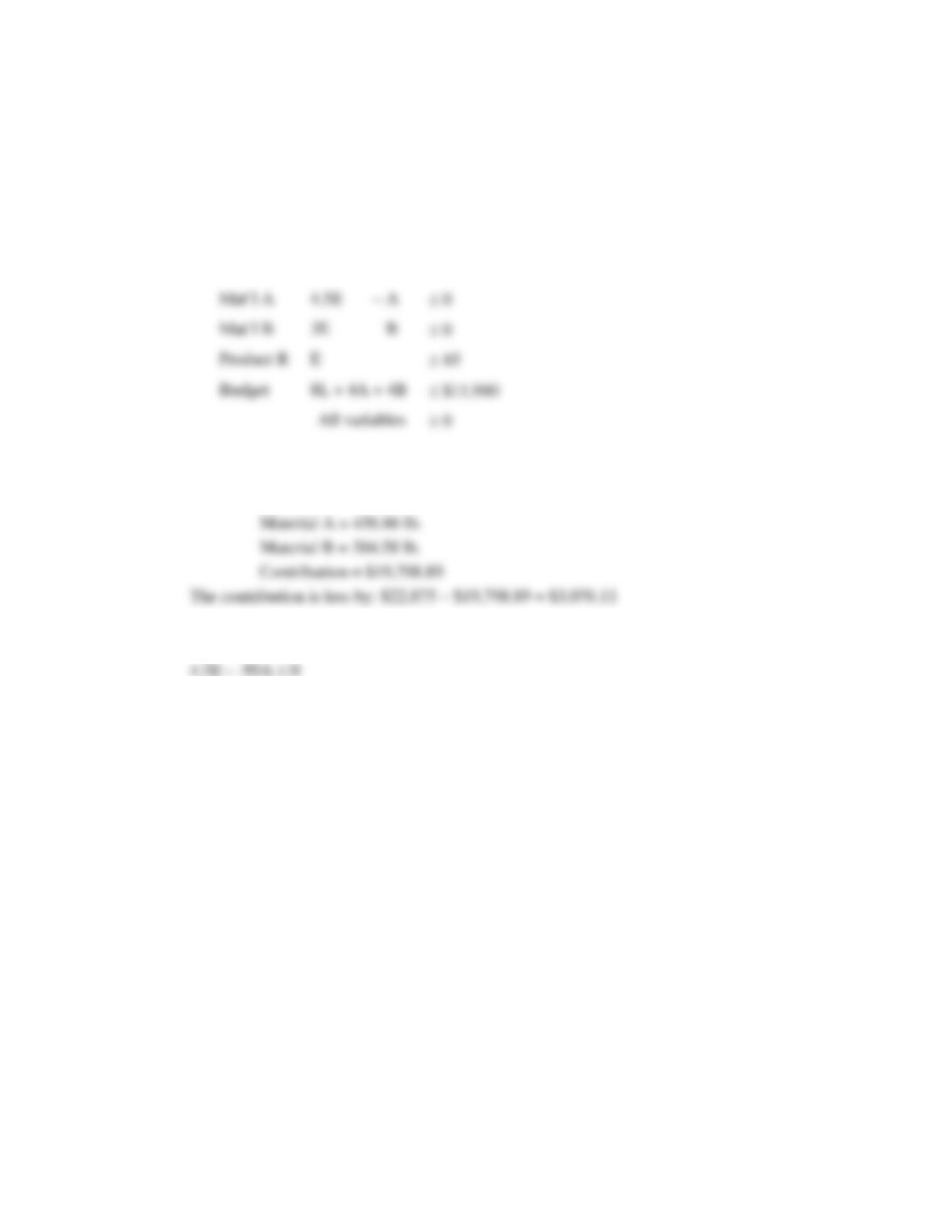
2. E = equal quantities of Q, R, and W
[E contribution is 122 + 115 + 76 = 313]
[An alternate approach would be T = total amount, with an average contribution of 313/3 =
104.333]
Maximize 313E – 8L – 4A – 4B
subject to
Labor
11E
– L
0
Optimal: E = 101.53 [i.e., Q = 101.53, R = 101.53, and W = 101.53.]
Labor = 1,116.78 hr.
3. 5% waste on A:
Product R
E
85
Chapter 19 – Linear Programming
19–17
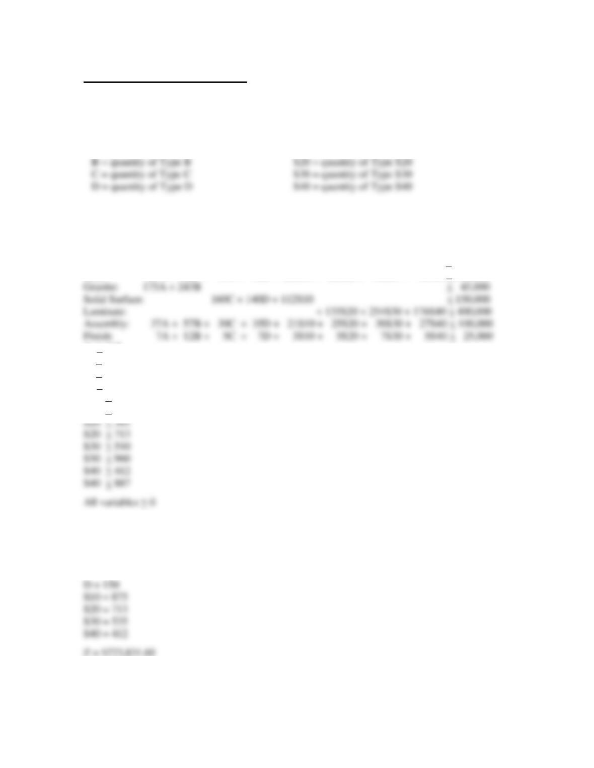
Case: Custom Cabinets, Inc.
Problem Formulation:
Semi-custom Cabinets Standard Cabinets
A = quantity of Type A S10 = quantity of Type S10
Max Z = 325A + 575B + 257C + 275D +175S10 + 210S20 + 260S30 + 230S40
s.t.
Wood: 125A + 160B + 140C + 200D + 60S10 + 110S20 + 200S30 + 180S40 < 400,000
Trim: 27A + 42B + 35C + 52D + 21S10 + 28S20 + 50S30 + 43S40 < 140,000
A > 117
B > 92
C > 130
D > 150
S10 > 475
S10 < 875
Optimal Values
A = 117
B = 101
C = 193
Chapter 19 – Linear Programming
19–18
Sensitivity Analysis
Both Assembly and Finishing have shadow prices equal to 0, so don’t work overtime.
Laminate also has a shadow price of 0, so don’t purchase additional laminate.
Wood has a shadow price of $1.30, and an allowable increase of 462,136.8 board feet. Purchase that
Enrichment Module: The Simplex Method
The simplex method is a general-purpose linear-programming algorithm widely used to solve large-
scale problems. Although it lacks the intuitive appeal of the graphical approach, its ability to handle
problems with more than two decision variables makes it extremely valuable for solving problems
often encountered in operations management.
When teaching the simplex method, please consider the following points:
1. A computer package for simplex is highly desirable because it permits assigning a range of
problems and concentrating on interpretation of solutions rather than on technique.
3. Insight receives a boost when simplex and graphical solutions are compared for the same
problem.
5. Minimization, artificial variables and ranging can be skipped without seriously impairing
appreciation and understanding of the simplex method.
The simplex technique involves a series of iterations; successive improvements are made until an
optimal solution is achieved. The technique requires simple mathematical operations (addition,
subtraction, multiplication, and division), but the computations are lengthy and tedious, and the
slightest error can lead to a good deal of frustration. For these reasons, most users of the technique rely
on computers to handle the computations while they concentrate on the solutions. Still, some