Excel Templates to accompany Operations Management, Eleventh Edition
created by Lee Tangedahl
Copyright © 2012 by The McGraw Hill Companies, Inc. All rights reserved.
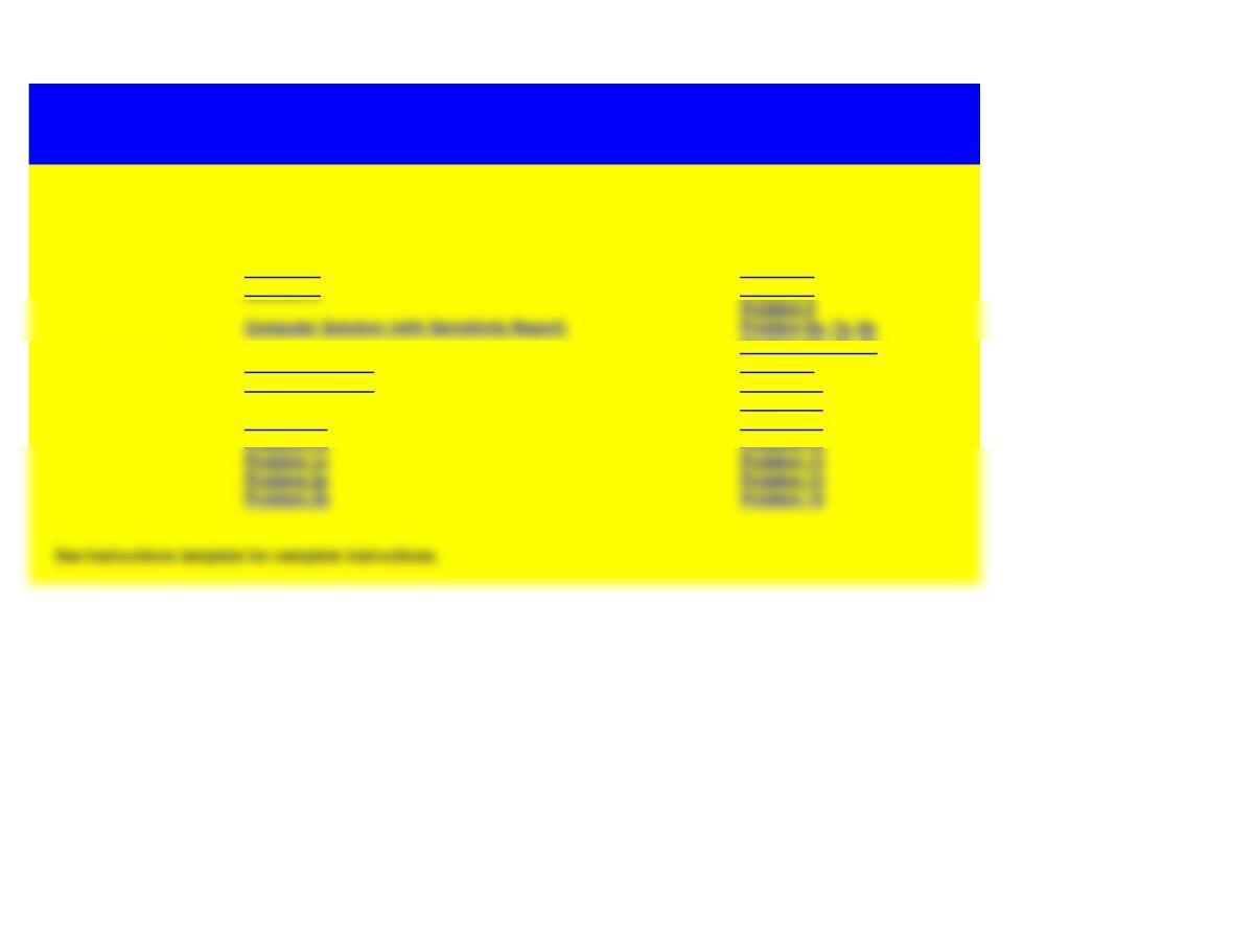
Chapter Nineteen – Linear Programming
These templates are each designed to demonstrate the solution for one particular problem only!
Examples: Example 2 Problems: Problem 3
Example 3 Problem 4
Problem 6b, 7b, 8b
Solved Problems: Solved Problem 1 Problem 9
Solved Problem 2 Problem 10
Problem 11
Problems: Problem 1a Problem 12
Problem 1b Problem 13
Problem 1c Problem 14
Problem 2a Problem 15
Problem 2b Problem 16
See Instructions template for complete instructions.
Problem 5
Computer Solution (with Sensitivity Report) Problem 6a, 7a, 8a
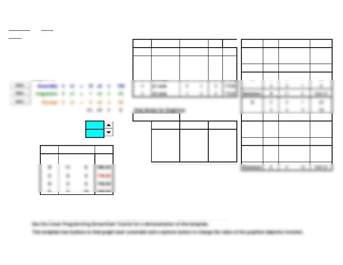
Example 2 Notes
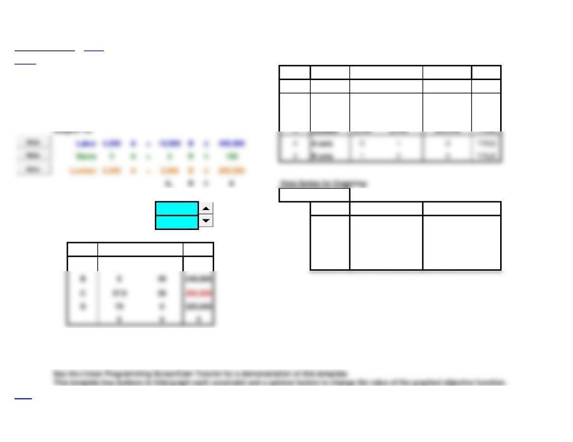
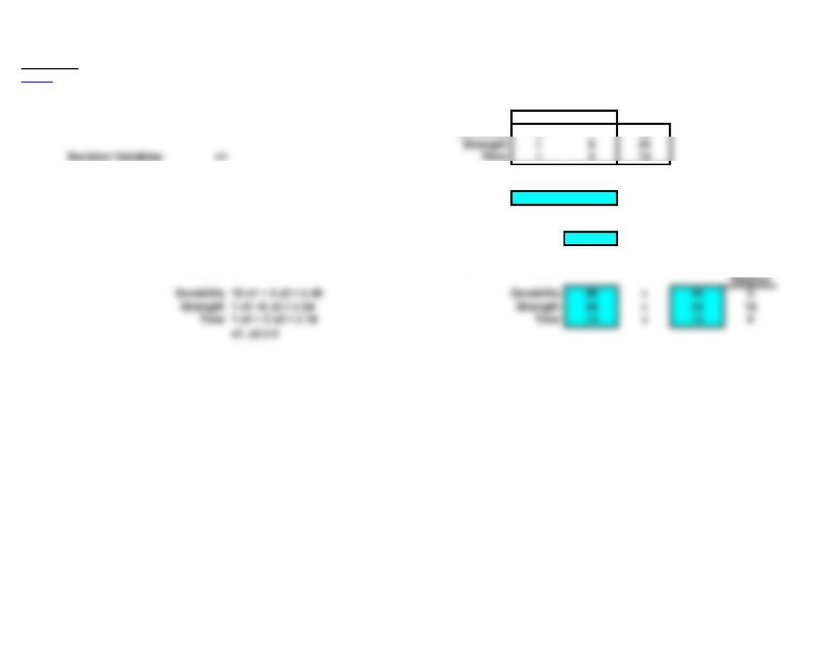
<Back Constraints: Solve for Solutions at Extreme Points:
x1 = quantity of type 1 to produce Number Name x1 x2 RHS Visible Point
Intersectio
x1 x2 RHS/Obj.
x2 = quantity of type 2 to produce Profit 60 50 300 TRUE A4 0 1 0
1Assembly 410 100 TRUE 5 1 0 0
Maximize 60 x1 +50 x2 = Profit 2Inspection 2 1 22 TRUE Solution: A 0 0 0.00
Subject To: 3Storage 3 3 39 TRUE B2 2 1 22
infinity = 10000000000 Solution: C 9 4 740.00
Graphed Profit = x1 x2 x1 x2 D1 4 10 100
Increment = Profit = 300 0 6 5 0 3 3 3 39
Assembly 0 10 25 0Solution: D 5 8 700.00
Point x1 x2 Profit Inspection 0 22 11 0E1 4 10 100
A 0 0 0.00 Storage 0 13 13 0 5 1 0 0
E 0 10 500.00
Notes:
This template is designed to demonstrate the graphical solution for this particular problem only.
300
10
<Top
E
9
10
11
12
13
14
15
22
23
24
25
x2
Example 2
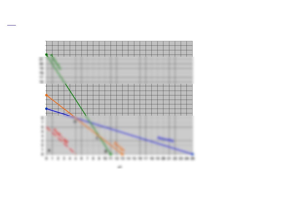
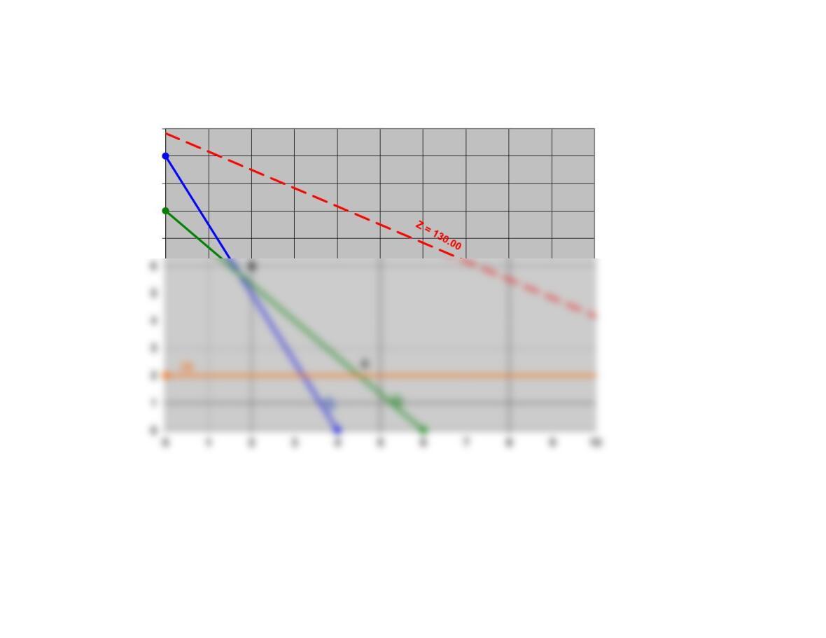
Example 3 Notes
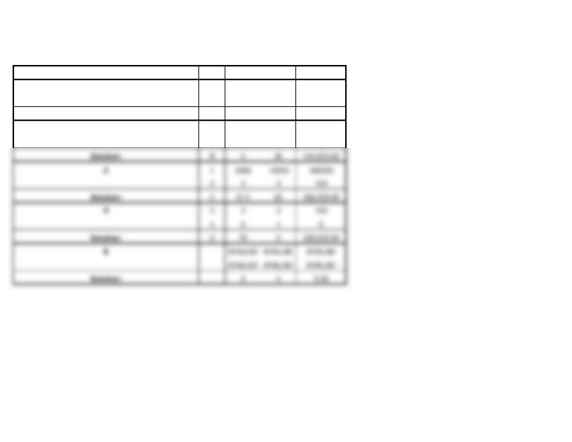
<Back Constraints:
x1Number Name x1 x2 RHS Visible
x2Z812 130 TRUE
1(1) 5 2 20 TRUE
8x1 +12 x2 = Z 2(2) 4 3 24 TRUE
max = 100
Graphed Z = x1 x2 x1 x2
Increment = Z = 130.00 0 10.83333333 16.25 0
(1) 0 10 4 0
Point x1 x2 Z(2) 0 8 6 0
A 0 10 120.00 (3) 0 2 100 2
130
5
Solve for Solutions at Extreme Points:
Point
Intersection
x1 x2 RHS/Obj.
A1 5 2 20
5 1 0 0
Solution:
A 0 10 120.00
B1 5 2 20
2 4 3 24
Notes:
This template is designed to demonstrate the graphical solution for this particular problem only.
See the Linear Programming ScreenCam Tutorial for a demonstration of this template.
Solution:
Solution:
Solution:
Solution:
A
7
8
9
10
11
Example 3
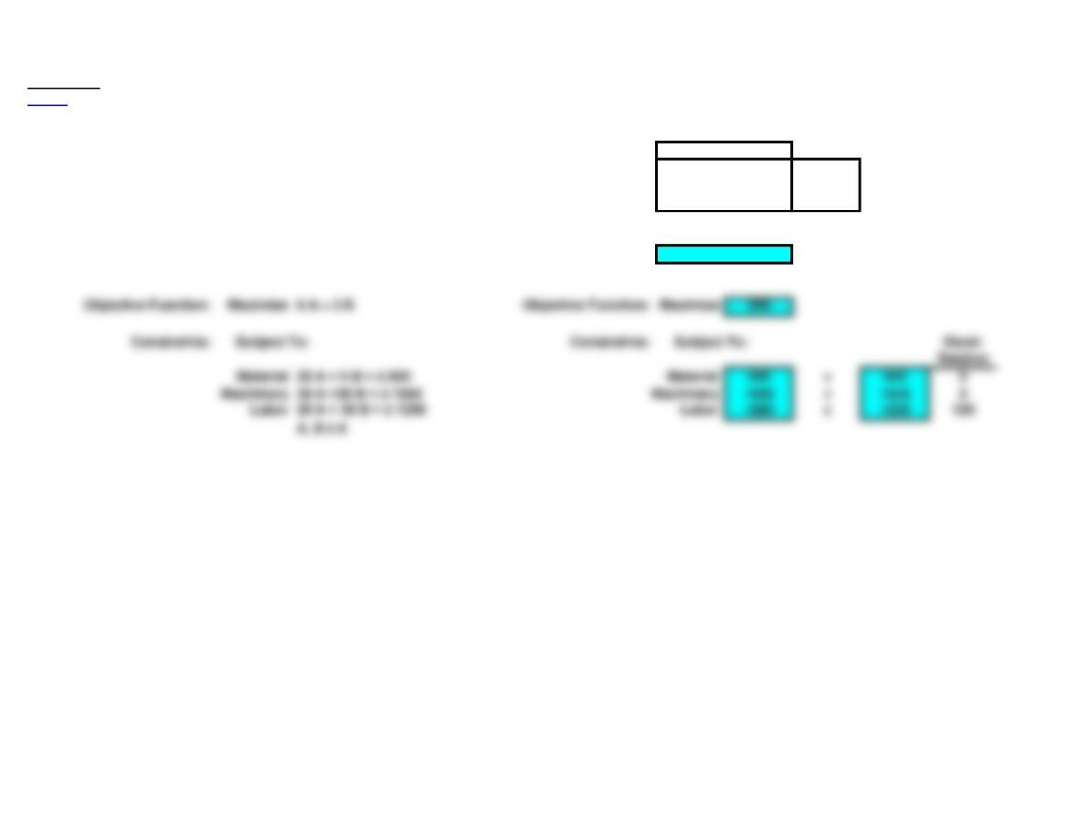
Computer Solution (with Sensitivity Report)
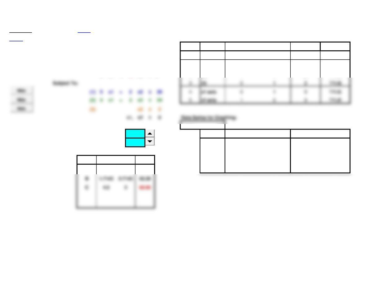
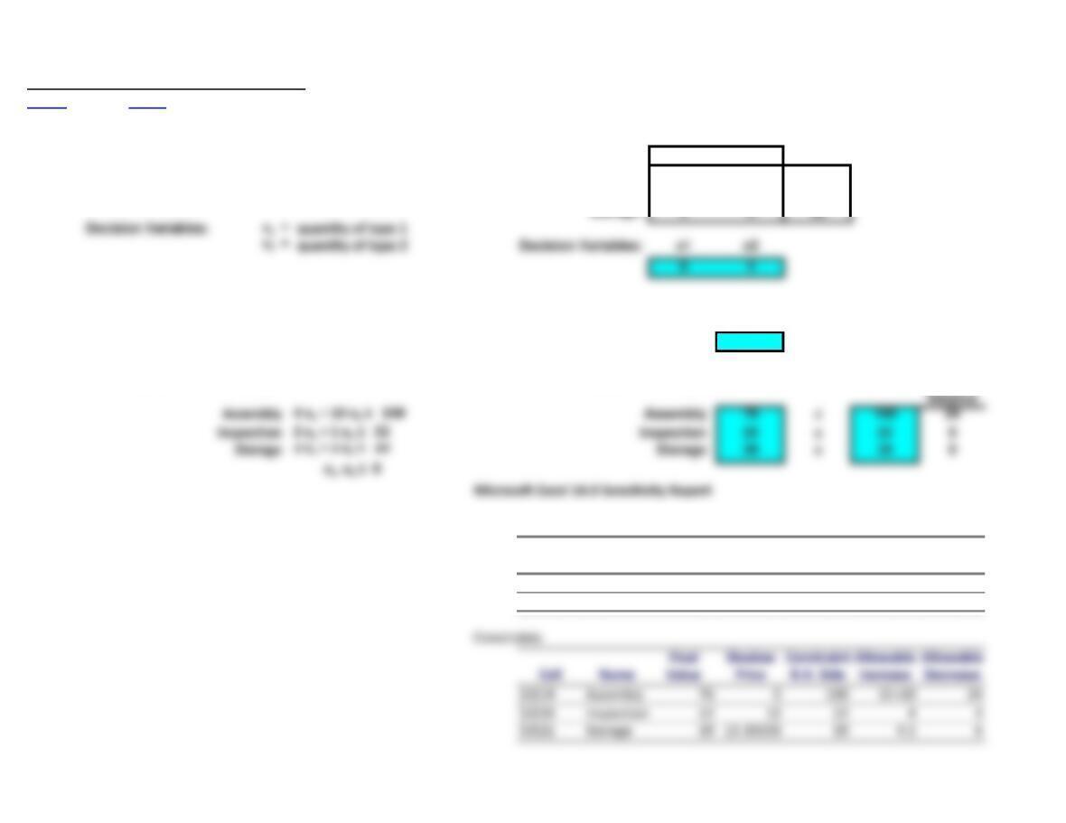
<Back Notes Solver Solution:
Model Formulation: Data:
x1 x2
Revenue per Unit 60 50 Available
Assembly 4 10 100
Inspection 2 1 22
Storage 3 3 39
Objective Function: Maximize 60 x1 + 50 x2Objective Function:
Maximize
740
Constraints: Subject To: Constraints: Subject To: Slack/
Variable Cells
Final Reduced Objective Allowable Allowable
Cell Name Value Cost
Coefficient
Increase Decrease
$I$11 x1 9 0 60 40 10
$J$11 x2 4 0 50 10 20
Notes:
This template is designed to demonstrate the Solver solution for this particular problem only.
See the Linear Programming ScreenCam Tutorial for a demonstration of this template.
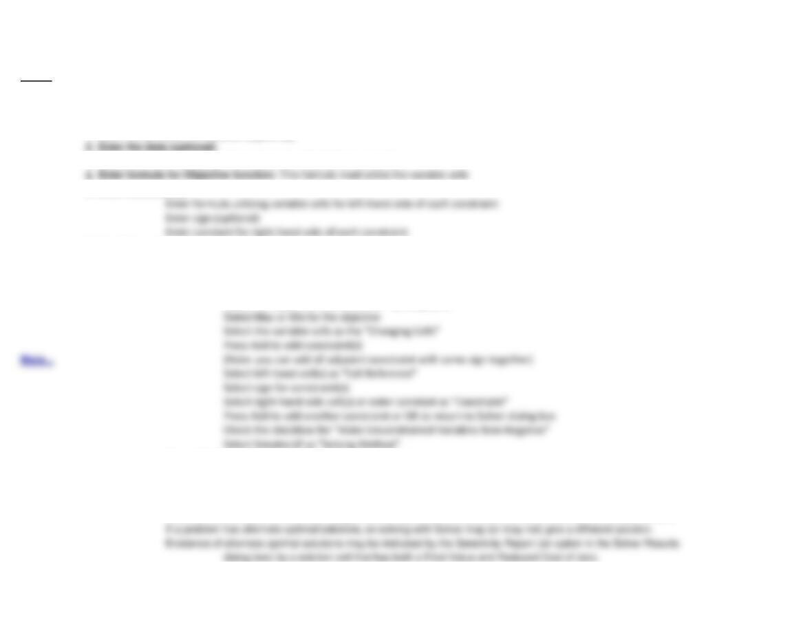
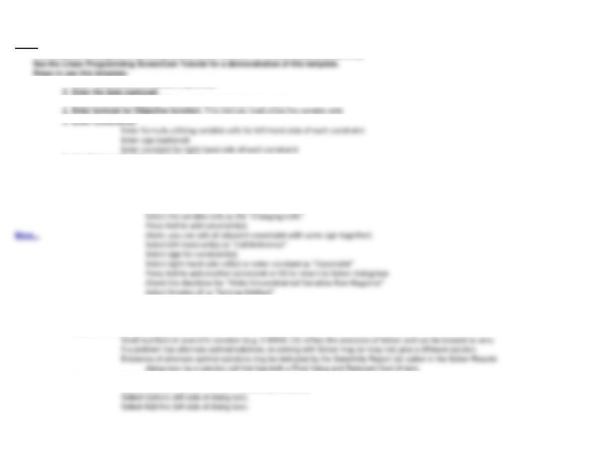
Steps to use this template:
1. Enter the problem formulation (optional)
3.
Create cells for variables: These cells are initially blank (or zero)
Enter formula for Objective function: This formula must utilize the variable cells
5. Enter Constraints:
Enter formula utilizing variable cells for left-hand-side of each constraint
Enter sign (optional)
Enter constant for right-hand-side of each constraint
6. Use Solver to find the optimal solution:
Select the Data ribbon, select Solver in the Analysis group.
(See note below to add-in Solve if it does not appear).
Enter parameters into Solver dialog box:
Select the objective function cell for “Set Objective:”
Select the variable cells as the “Changing Cells”
Press Add to add constraint(s)
(Note: you can add all adjacent constraint with same sign together)
Select left-hand-cell(s) as “Cell Reference”
Select sign for constraint(s)
Select right-hand-side cell(s) or enter constant as “Constraint”
Press Add to add another constraint or OK to return to Solver dialog box
Check the checkbox for “Make Unconstrained Variables Non-Negative”
Select Simplex LP as “Solving Method”
Press Solve
Read message in Solver Results dialog box.
Select Answers and/or Sensitivity Report(s) (optional)
Press OK
Notes on the Solver solution:
Small numbers in scientific notation (e.g. 2.4091E-11) reflect the precision of Solver and can be treated as zero.
How to Add-In Solver if it does not appear in the Analysis group of the Data ribbon:
Select File (left-most item in main menu at top of screen).
Solved Problem 1 Notes
<Back Constraints:
A = number of type A houses to build Number Name A B RHS Visible
B = number of type B houses to build Profit 3,000 6,000 100,000 TRUE
1Labor 4,000 10,000 400,000 TRUE
Maximize 3,000 A + 6,000 B = Profit 2Stone 2 3 150 TRUE
infinity = 1E+10
Graphed Profit = A B A B
Increment =
Profit = 1000
016.66666667 33.33333333 0
Labor 040 100 0
Point A B Profit Stone 0 50 75 0
A 0 0 0 Lumber 0 100 100 0
Notes:
This template is designed to demonstrate the graphical solution for this particular problem only.
<Top
100,000
10,000
Solve for Solutions at Extreme Points:
Point
Intersectio
A B RHS/Obj.
A4 0 1 0
5 1 0 0
Solution: A 0 0 0.00
B14000 10000 400000
5 1 0 0
70
80
90
100
110
A
Solved Problem 1
Solved Problem 2
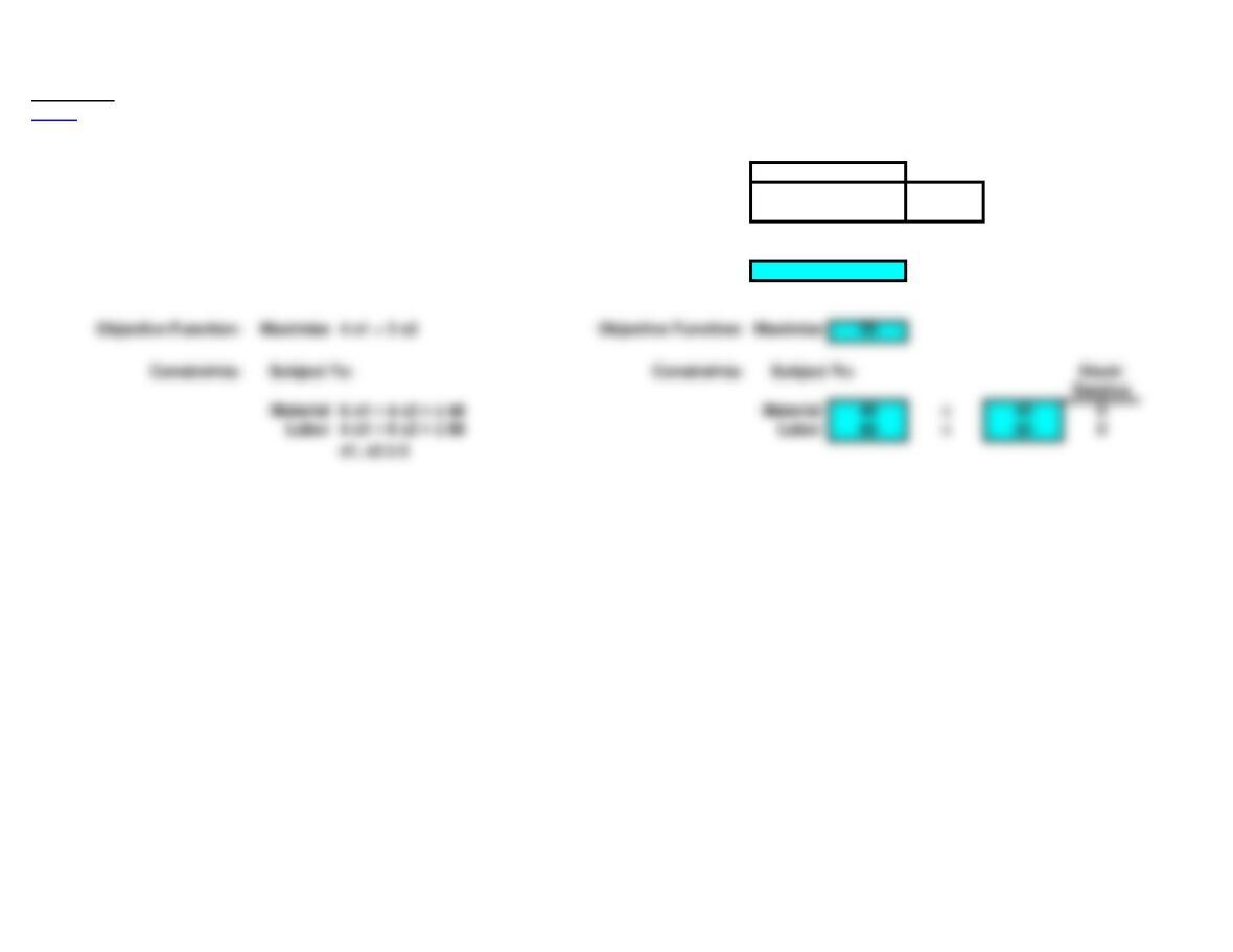
<Back Notes Solver Solution:
Model Formulation: Data:
x1x2x3
Profit per Unit 15 20 14
Labor 5 6 4 210
Material 10 8 5 200
Machine 4 2 5 170
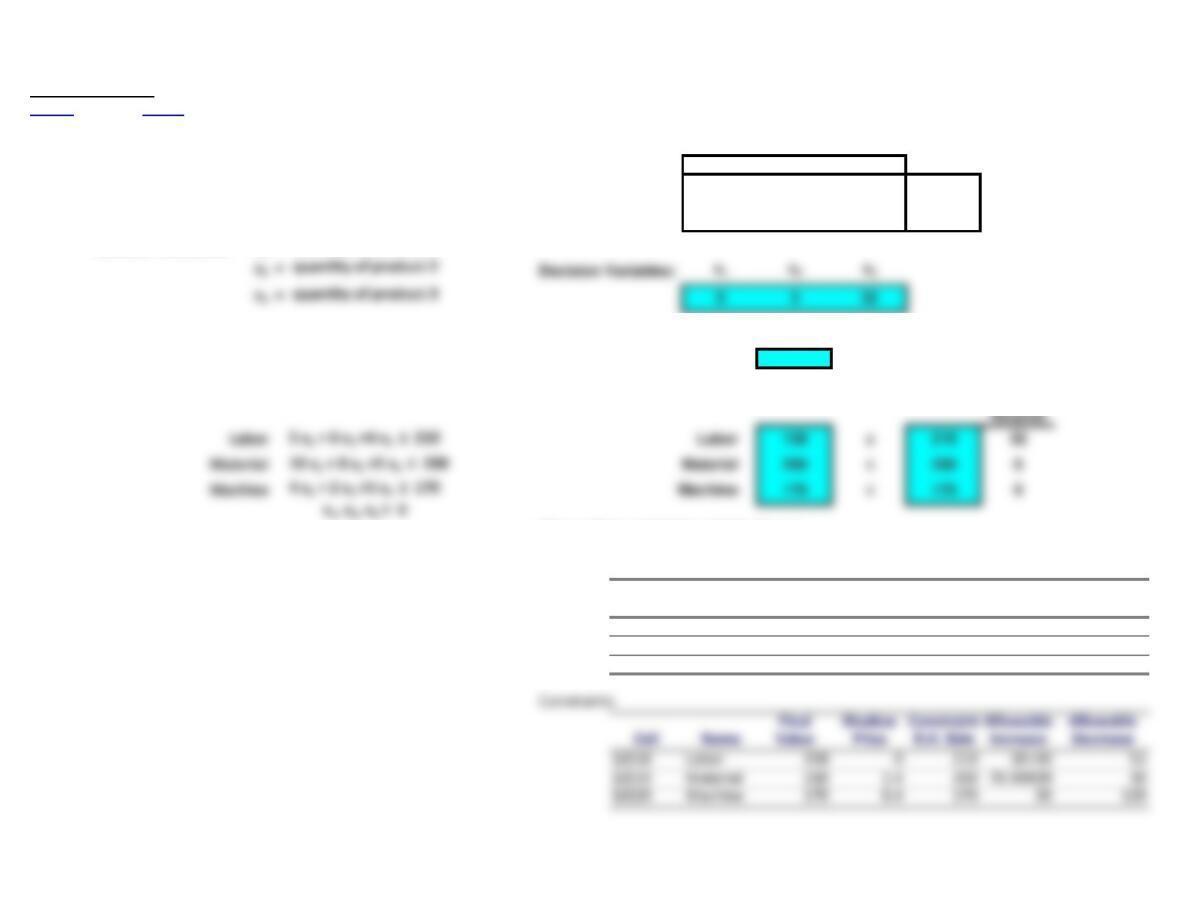
Decision Variables:
x1 =
quantity of product 1
Objective Function:
ximize
15 x1 + 20 x2 + 14 x3Objective Function:
Maximize
548
Constraints: Subject To: Constraints: Subject To: Slack/
4 x1 + 2 x2 +5 x3 ≤ 170 Machine 170 ≤170 0
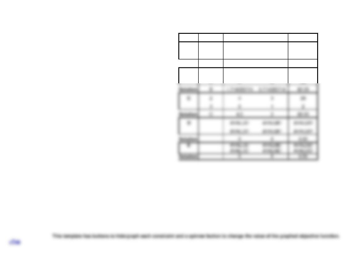
Microsoft Excel 14.0 Sensitivity Report
Variable Cells
Final Reduced Objective Allowable Allowable
Cell Name Value Cost
Coefficient
Increase Decrease
$I$11
quantity o
0 -10.6 15 10.6 1E+30
$J$11
quantity o
5 0 20 2.4 10.6
$K$11
quantity o
32 014 36 1.5
Notes:
This template is designed to demonstrate the Solver solution for this particular problem only.
1. Enter the problem formulation (optional)
2. Enter the data (optional)
3. Create cells for variables: These cells are initially blank (or zero)
4.
5. Enter Constraints:
6. Use Solver to find the optimal solution:
Select the Data ribbon, select Solver in the Analysis group.
(See note below to add-in Solve if it does not appear).
Enter parameters into Solver dialog box:
Select the objective function cell for “Set Objective:”
Select Max or Min for the objective
Select the variable cells as the “Changing Cells”
Press Add to add constraint(s)
Select left-hand-cell(s) as “Cell Reference”
Select sign for constraint(s)
Select right-hand-side cell(s) or enter constant as “Constraint”
Press Add to add another constraint or OK to return to Solver dialog box
Check the checkbox for “Make Unconstrained Variables Non-Negative”
Select Simplex LP as “Solving Method”
Press S
Read message in Solver Results dialog box.
Select Answers and/or Sensitivity Report(s) (optional)
Press OK
Notes on the Solver solution:
If a problem has alternate optimal solutions, re-solving with Solver may (or may not) give a different solution.
Existence of alternate optimal solutions may be indicated by the Sensitivity Report (an option in the Solver Results
dialog box) by a solution cell that has both a Final Value and Reduced Cost of zero.
How to Add-In Solver if it does not appear in the Analysis group of the Data ribbon:
Select File (left-most item in main menu at top of screen).
Select Options (left side of dialog box).
See the Linear Programming ScreenCam Tutorial for a demonstration of this template.
Steps to use this template:
Problem 1a
<Back Solver Solution:
Model Formulation: Data:
x1 x2
Z 4 3
Material 6 4 48
Decision Variables: x1 Labor 4 8 80
x2
Decision Variables: x1 x2
2 9
Problem 1b
<Back Solver Solution:
Model Formulation: Data:
x1 x2
Z 210
Durability 10 440
x2
Decision Variables: x1 x2
1.5 6.25
Objective Function: Maximize 2 x1 + 10 x2 Objective Function: Maximize 65.5
Constraints: Subject To: Constraints: Subject To: Slack/
Problem 1c
<Back Solver Solution:
Model Formulation: Data:
A B
Z 6 3
Material 20 6600
Machinery 25 20 1,000
Decision Variables: A Labor 20 30 1,200
B
Decision Variables: A B
24 20