Chapter 19 – Linear Programming
19–19
Maximize
Z =
4x1
+ 5x2
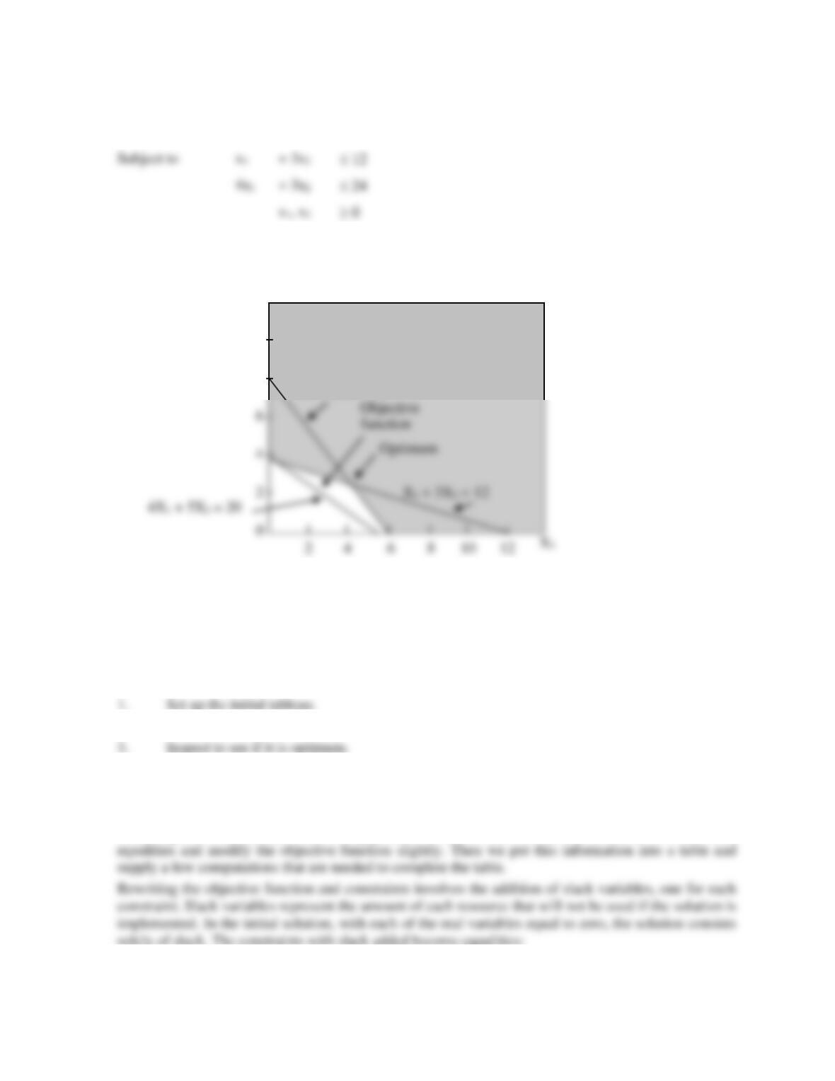
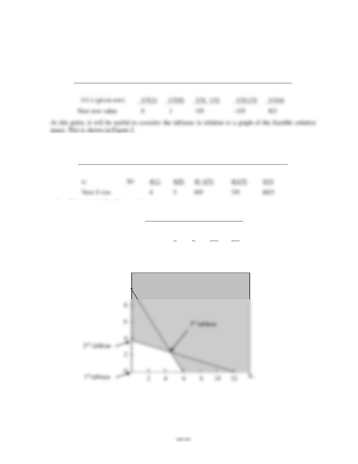
The solution is shown graphically in Figure 1. Now let’s see how the simplex technique can be used to
obtain the solution.
Figure 1. Graphical Solution
X1 + 3X2 = 12
The simplex technique involves generating a series of solutions in tabular form, called tableaus. By
inspecting the bottom row of each tableau, one can immediately tell if it represents the optimal
solution. Each tableau corresponds to a corner point of the feasible solution space. The first tableau
corresponds to the origin. Subsequent tableaus are developed by shifting to an adjacent corner point in
the direction that yields the highest rate of profit. This process continues as long as a positive rate of
profit exists. Thus, the process involves the following steps:
2. Develop a revised tableau using the information contained in the first tableau.
4. Repeat steps 2 and 3 until no further improvement is possible.
Setting Up the Initial Tableau
Obtaining the initial tableau is a two-step process. First, we must rewrite the constraints to make them
10
8
X2
4X1 + 3X2 = 24
Chapter 19 – Linear Programming
19–20
1)
x1
+ 3x2
+ 1s1
= 12
2)
4x1
+ 3x2
+ 1s2
= 24
The objective function can be written in similar form:
Z = 4x1 + 5x2 + 0s1 + 0s2
The slack variables are given coefficients of zero in the objective function because they do not
produce any contributions to profits. Thus, the information above can be summarized as:
+ 3x2
+ 1s1
+ 0s2
= 12
+ 3x2
+ 0s1
+ 1s2
= 24
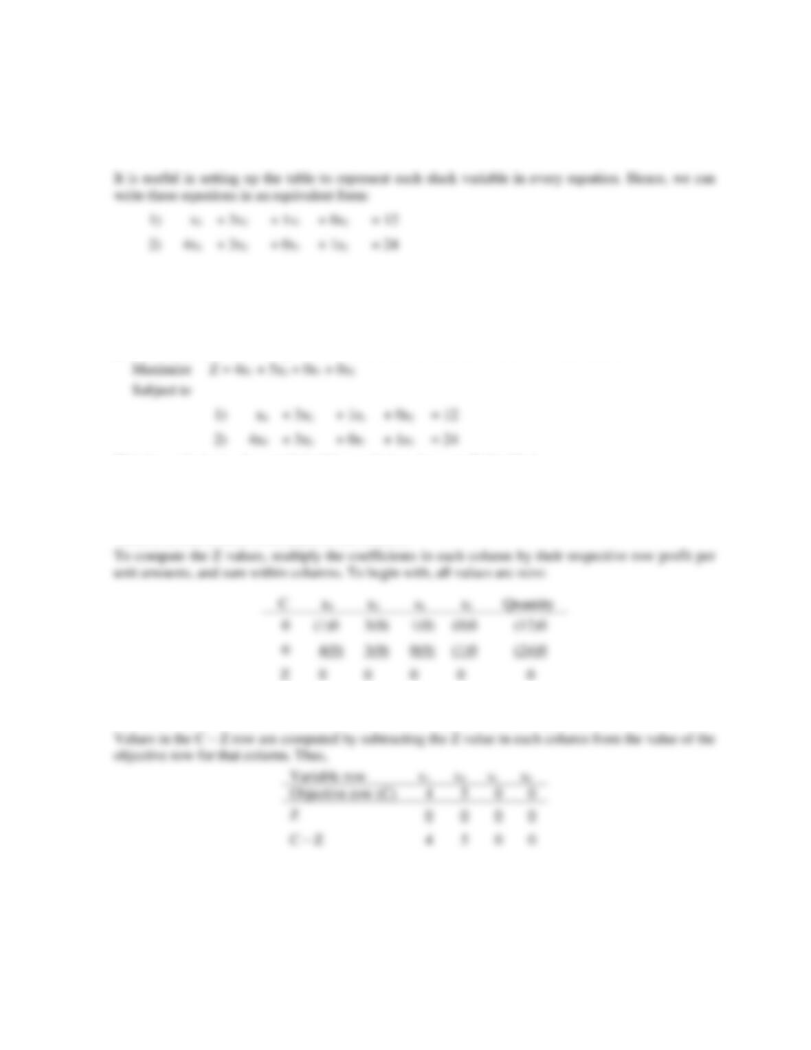
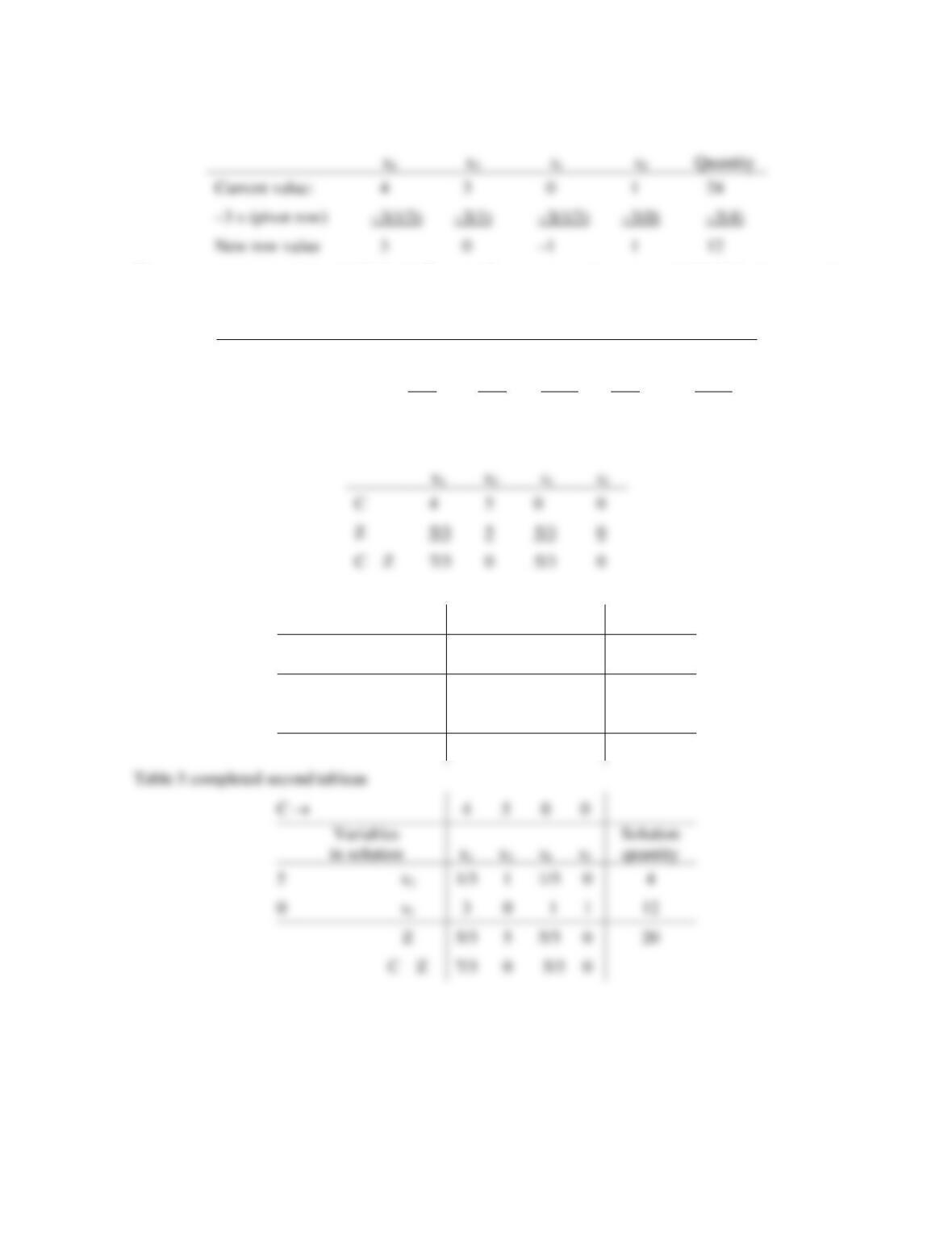
This forms the basis of our initial tableau, which is shown in Table 5S–1.
To complete the first tableau, we will need two additional rows, a Z row and a C – Z row. The Z row
values indicate the reduction in profit that would occur if one unit of the variable in that column were
added to the solution. The C – Z row shows the potential for increasing profit if one unit of the
variable in that column were added to the solution.
The last value in the Z row indicates the total profit associated with a given solution (tableau). Since
the initial solution always consists of the slack variables, it is not surprising that profit is 0.
Z
1)
+ 3x2
+ 1s1
+ 0s2
= 12
2)
+ 3x2
+ 0s1
+ 1s2
= 24
Chapter 19 – Linear Programming
19–21
Table 1 Partial Initial Tableau
Profit per unit
for variables
in solution
Decision
Variables
C
4
5
0
0
Objective
row
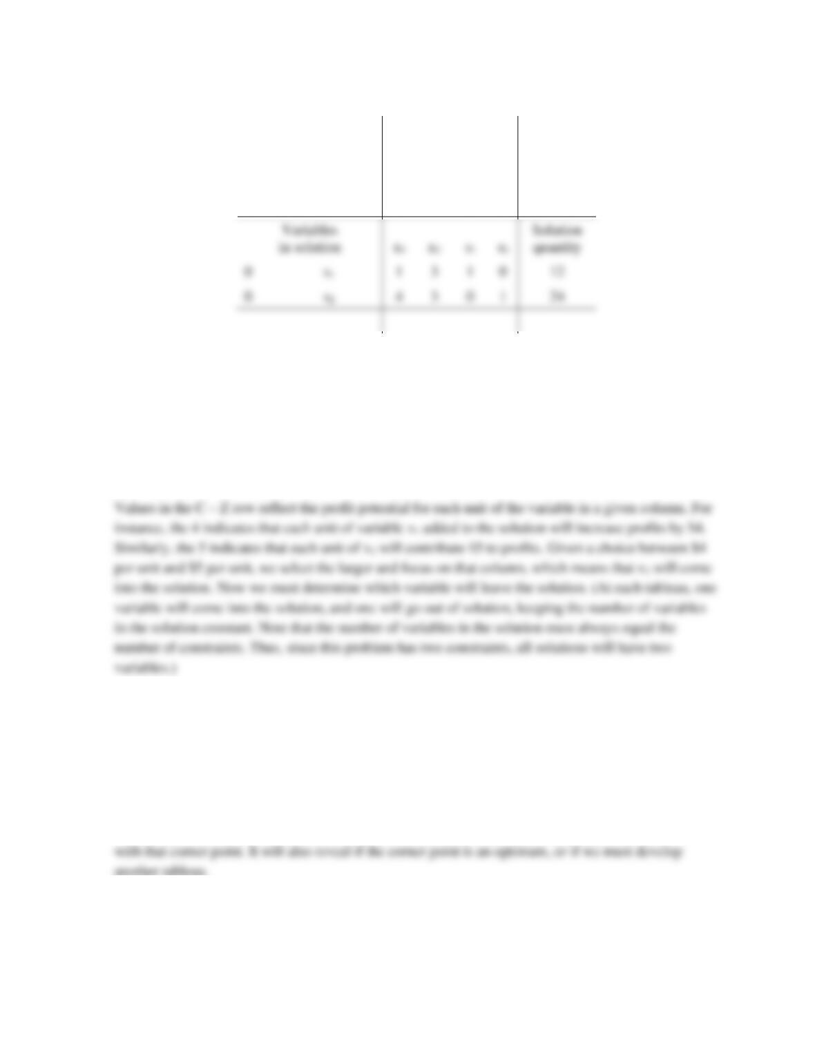
The completed tableau is shown in Table 2.
The Test for Optimality
If all the values in the C – Z row of any tableau are zero or negative, the optimal solution has been
obtained. In this case, the C – Z row contains two positive values, 4 and 5, indicating that
improvement is possible.
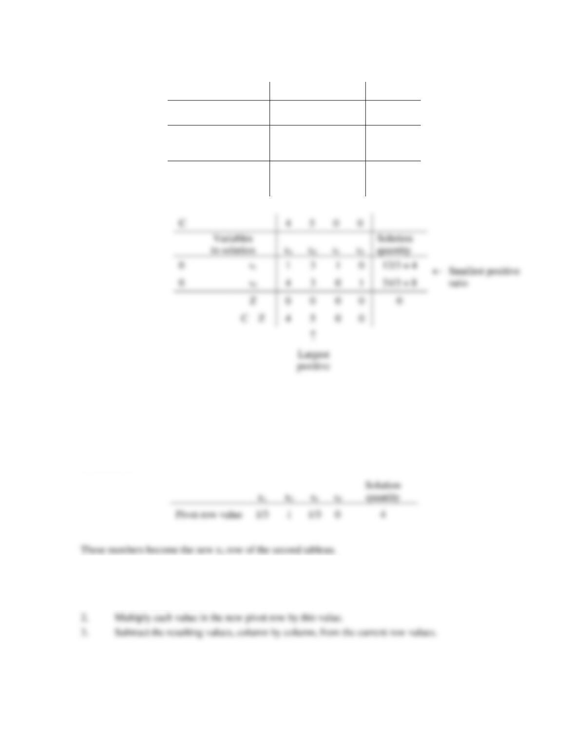
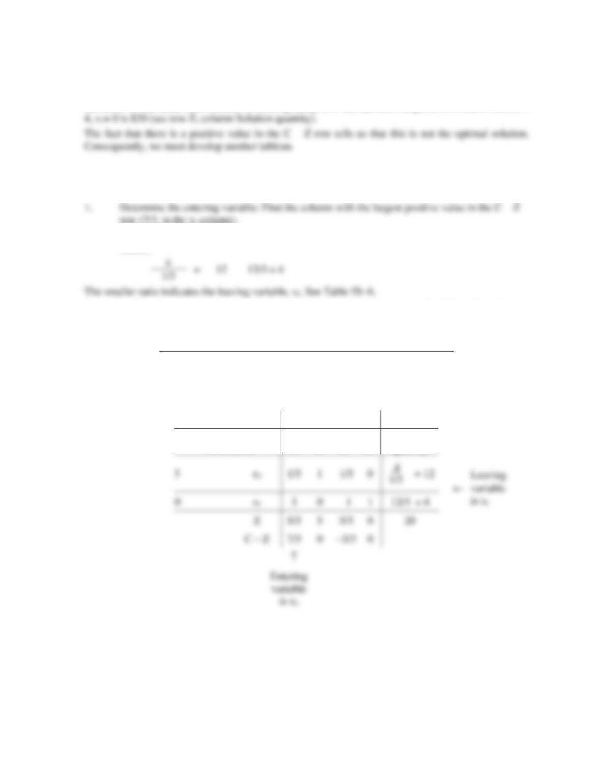
Developing the Second Tableau
To determine which variable will leave the solution, we use the numbers in the body of the table in the
column of the entering variable (i.e., 3 and 3). These are called row pivot values. Divide each one into
the corresponding solution quantity amount, as shown in Table 3. The smaller of these two ratios
indicates the variable that will leave the solution. Thus, variable s1 will leave and be replaced with x2.
In graphical terms, we have moved up the x2 axis to the next corner point. By determining the smallest
ratio, we have found which constraint is the most limiting. In Figure 1, note that the two constraints
intersect the x2 axis at 4 and 8, the two row ratios we have just computed. The second tableau will
describe the corner point where x2 = 4 and x1 = 0; it will indicate the profits and quantities associated
0
0
4
3
0
1
Chapter 19 – Linear Programming
19–22
Table 2 Completed Initial Tableau.
C →
4
5
0
0
Variables
in solution
x1
x2
s1
s2
Solution
quantity
0
s1
1
3
1
0
12
0
s2
4
3
0
1
24
Z
0
0
0
0
0
C – Z
4
5
0
0
At this point we can begin to develop the second tableau. The row of the leaving variable will be
transformed into the new pivot row of the second tableau. This will serve as a foundation on which to
develop the other rows. To obtain this new pivot row, we simply divide each element in the s1 row by
the row pivot value (intersection of the entering column and leaving row), which is 3. The resulting
numbers are:
The pivot-row numbers are used to compute the values for the other constraint rows (in this instance,
the only other constraint row is the s2 row). The procedure is:
1. Find the value that is at the intersection of the constraint row (i.e., the s2 row) and the entering
variable column. It is 3.
Variables
in solution
x1
x2
s1
s2
Solution
quantity
0
s1
1
3
1
0
12/3 = 4
0
s2
4
3
0
1
24/3 = 8
Z
0
0
0
0
0
C – Z
4
5
0
0
Chapter 19 – Linear Programming
19–23
The two new rows are shown in Table 4. The new Z row can now be computed. Multiply the row unit
profits and the coefficients in each column for each row. Sum the results within each column. Thus,
Row
Profit
x1
x2
s1
s2
Quantity
x2
5
5(1/3)
5(1)
5(1/3)
5(0)
5(4)
s1
0
0(3)
0(0)
0(–1)
0(1)
0(12)
New Z row
5/3
5
5/3
0
20
Next, we compute the C – Z row:
C
4
5
0
0
Z
Table 4 partially completed second tableau
C
4
5
0
0
Variables
in solution
x1
x2
s1
s2
Solution
quantity
5
x2
1/3
3
1/3
0
4
0
s2
3
0
–1
1
12
4
5
0
0
1/3
1
0
3
0
1
5/3
5
0
20
7/3
0
0
Current value:
Chapter 19 – Linear Programming
19–24
The completed second tableau is shown in Table 5. It tells us that at this point 4 units of variable x2 are
the most we can make (see column Solution quantity, row x2) and that the profit associated with x2 =
Developing the Third Tableau
The third tableau will be developed in the same manner as the previous one.
2. Determine the leaving variable: Divide the solution quantity in each row by the row pivot.
Hence,
4
1/3
3. Divide each value in the row of the leaving variable by the row pivot value (3) to obtain the
new pivot-row values:
x1
x2
s1
s2
Quantity
Current value
3
0
–1
1
12
New pivot-row value
1
0/3
–1/3
1/3
12/3 = 4
Table 6 Leaving/Entering Variables
C
4
5
0
0
Variables
in solution
x1
x2
s1
s2
Solution
quantity
5/3
Chapter 19 – Linear Programming
4. Compute values for the x2 row: Multiply each new pivot-row value by the x2 row pivot value
(i.e., 1/3) and subtract the product from corresponding current values. Thus,
x1
x2
s1
s2
Quantity
Current value:
1/3
1
1/3
0
4
5. Compute new Z row values. Note that now variable x1 has been added to the solution mix; that
row’s unit profit is $4.
Row
Profit
x1
x2
s1
s2
Quantity
x2
$5
5(0)
5(1)
5(4/9)
5(–1/9)
5(8/3)
x1
$4
4(1)
4(0)
4(–1/3)
4(1/3)
4(4)
New Z row
8/9
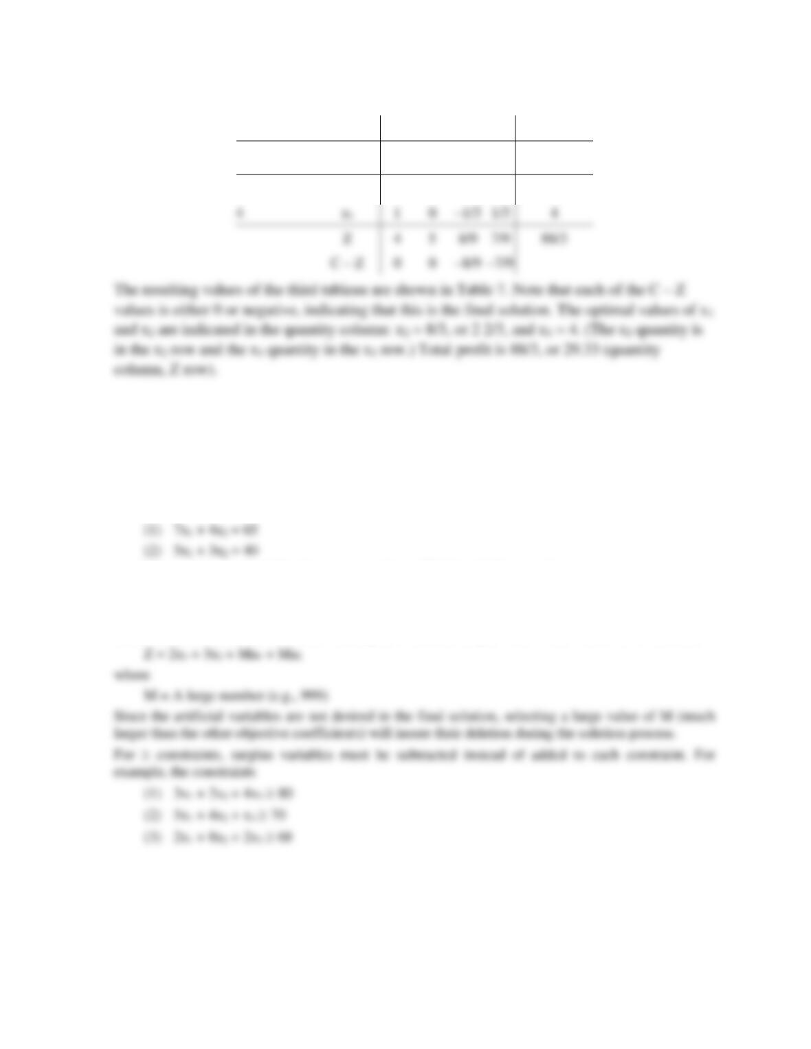
6. Compute the C – Z row values:
x1
x2
s1
s2
C
4
5
0
0
Z
4
5
8/9
7/9
C – Z
0
0
–8/9
–7/9
Figure 2 Graphical Solution and Simplex Tableaus
10
X2
Chapter 19 – Linear Programming
19–26
Table 7. Optimal Solution
C
4
5
0
0
Variables
in solution
x1
x2
s1
s2
Solution
quantity
5
x2
0
1
4/9
–1/9
8/3
Handling and = Constraints
Up to this point, we have worked with constraints. Constraints that involve equalities and
constraints are handled in a slightly different way.
When an equality constraint is present, use of the simplex method requires addition of an artificial
variable. The purpose of such variables is merely to permit development of an initial solution. For
example, the equalities
would be rewritten in the following manner using artificial variables a1 and a2:
(1) 7x1 + 4x2 + 1a1 + 0a2 = 65
(2) 5x1 + 3x2 + 0a1 + 1a2 = 40
Slack variables would not be added. The objective function, say Z = 2x1 + 3x2, would be rewritten as:
4
1
4
5
8/9
0
Chapter 19 – Linear Programming
19–27
would be rewritten as equalities:
(1) 3x1 + 2x2 + 4x3 – 1s1 – 0s2 – 0s3 = 80
As equalities, each constraint must then be adjusted by inclusion of an artificial variable. The final
result looks like this:
(1) 3x1 + 2x2 + 4x3 – 1s1 – 0s2 – 0s3 + 1a1 + 0a2 + 0a3 = 80
If the objective function happened to be
5x1 + 2x2 + 7x3
Summary of Maximization Procedure
The main steps in solving a maximization problem with only constraints using the simplex algorithm
are these:
1. Set up the initial tableau.
of 0.
c. Put the objective coefficients and constraint coefficients into tableau form.
2. Set up subsequent tableaus.
a. Determine the entering variable (the largest positive value in the C– Z row). If a tie exists,
choose one column arbitrarily.
c. Form the new pivot row of the next tableau: Divide each number in the leaving row by the
row’s pivot value. Enter these values in the next tableau in the same row positions.
d. Compute new values for remaining constraint rows: For each row, multiply the values in the
new pivot row by the constraint row’s pivot value, and subtract the resulting values, column by
column, from the original row values. Enter these in the new tableau in the same positions as
the original row.
Chapter 19 – Linear Programming
19–28
constraints, which requires both artificial variables and surplus variables. This tends to make manual
solution more involved. A second major difference is the test for the optimum: A solution is optimal if
there are no negative values in the C – Z row.
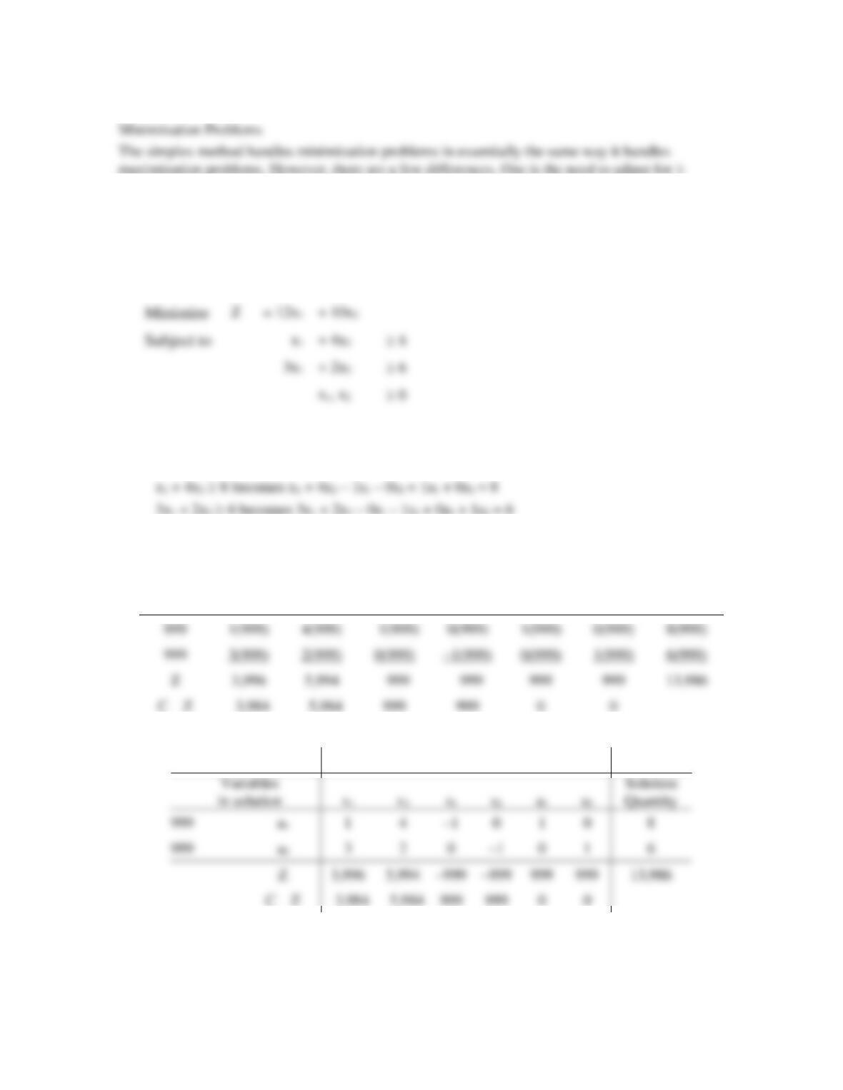
Example
Solve the following problem for the quantities of x1 and x2 that will minimize cost.
Solution to example
1. Rewrite the constraints so that they are in the proper form:
2. Rewrite the objective function (coefficients of C row):
12x1 + 10x2 + 0s1 + 0s2 + 999a1 + 999a2
3. Compute values for rows Z and C – Z:
C
x1
x2
s1
s2
a1
a2
Quantity
4. Set up the initial tableau. (Note that the initial solution has all artificial variables.)
C
12
10
0
0
999
999
999
0
1
0
3,996
5,994
999
999
13,986
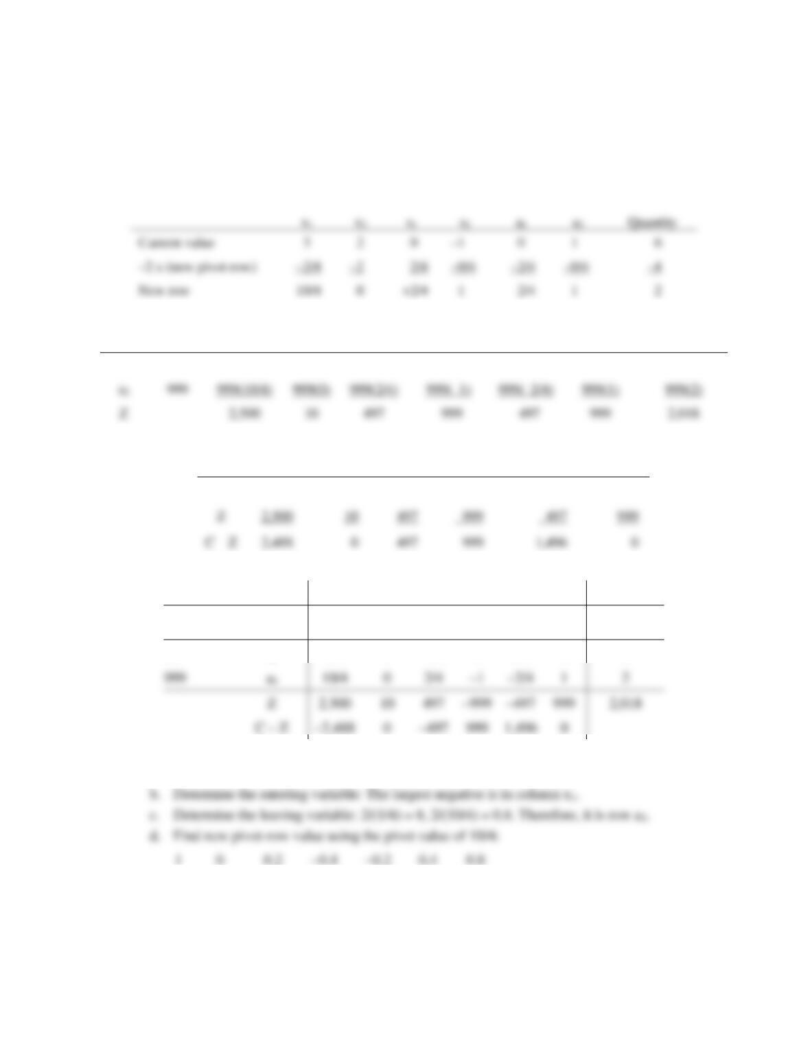
5. Find the entering variable (largest negative C – Z value: x2 column) and leaving variable
(smaller of 8/4 = 2 and 6/2 =3; hence, row a1).
Chapter 19 – Linear Programming
19–29
6. Divide each number in the leaving row by the pivot value (4, in this case) to obtain values for
the new pivot row of the second tableau:
1/4
4/4 = 1
–1/4
0/4
1/4
0/4
8/4 = 2
7. Compute values for other rows; a2 is:
8. Compute a new Z row:
Row
Cost
x1
x2
s1
s2
a1
a2
Quantity
x2
10
10(1/4)
10(1)
10(–1/4)
10(0)
10(1/4)
10(0)
10(2)
9. Compute the C – Z row:
x1
x2
s1
s2
a1
a2
C
12
10
0
0
999
999
Z
10
497
999
0
999
0
10. Set up the second tableau:
C
12
10
0
0
999
999
Variables
in solution
x1
x2
s1
s2
a1
a2
Solution
Quantity
10
a1
1/4
1
–1/4
0
1/4
0
2
999
a2
0
2/4
–2/4
1
2
2,500
10
497
999
0
999
0
11. Repeat the process.
a. Check for optimality: It is not optimum because of negatives in C – Z row.
s2
a2
Quantity
2/4
Chapter 19 – Linear Programming
19–30
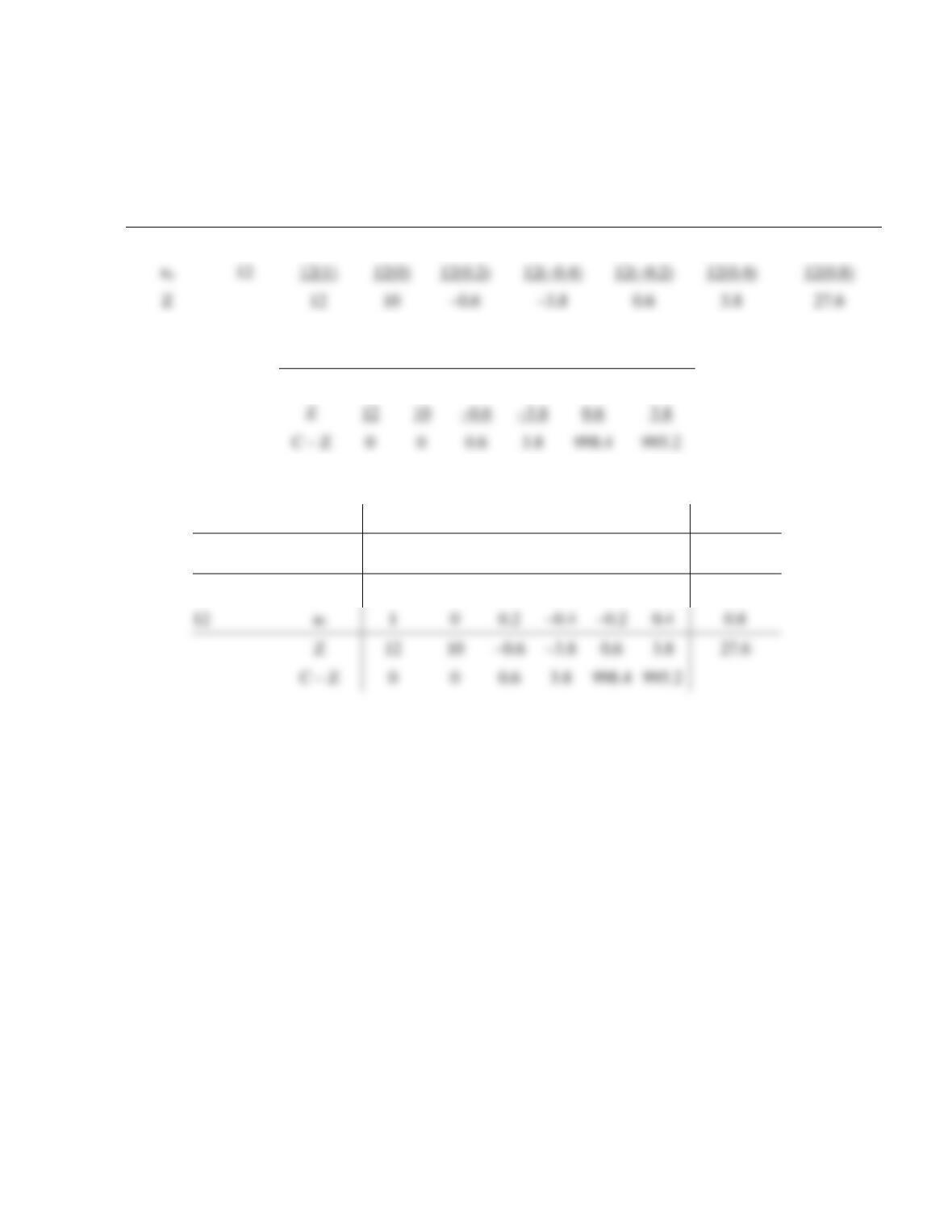
e. Determine values for new x2 row:
0
1
–0.3
0.1
0.3
–0.1
1.8
f. Determine new values for row Z:
Row
Cost
x1
x2
s1
s2
a1
a2
Quantity
x2
10
10(0)
10(1)
10(–0.3)
10(0.1)
10(0.3)
10(–0.1)
10(1.8)
g. Determine values for the C – Z row:
x1
x2
s1
s2
a1
a2
C
12
10
0
0
999
999
–3.8
0
0
0.6
h. Set up the next tableau. Since no C – Z values are negative, the solution is optimal. Hence,
x1 = 0.8, x2 = 1.8, and minimum cost is 27.60.
C
12
10
0
0
999
999
Variables
in solution
x1
x2
s1
s2
a1
a2
Quantity
10
a1
0
1
–0.3
0.1
0.3
–0.1
1.8
12
1
0
0.2
–0.6
0.6
3.8
0
0
0.6
x1
12
12(1)
12(0)
12(0.2)
12(0.4)
12(0.8)
3.8
Chapter 19 – Linear Programming
19–31
Problems for the enrichment module (simplex)
1. Given this information:
Maximize
Z = 10.50x + 11.75y + 10.80z
Subject to
2. Use the simplex method to solve these problems:
a.
Minimize
Z = 21x1 + 18x2
b.
Minimize
Z = 2x + 5y + 3z
3. Use the simplex method to solve the following problem.
Minimize Z = 3x1 + 4x2 + 8x3
4. Use the simplex method to solve the following problem.
Maximize Z = 8x1 + 2x2
Chapter 19 – Linear Programming
19–32
Solutions-Enrichment Module (SIMPLEX)
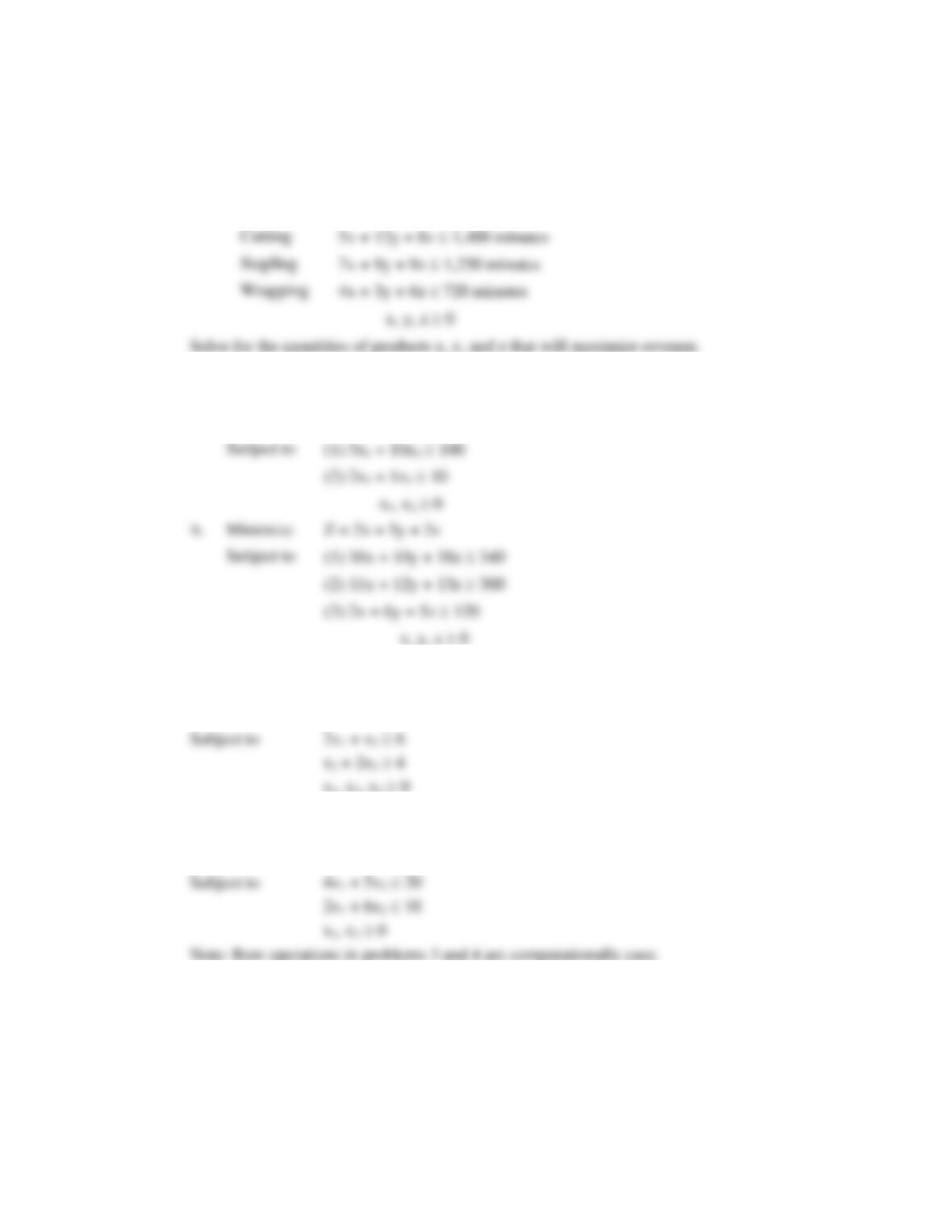
1.
C
10.5
11.75
10.80
0
0
0
Var
x
y
z
S1
S2
S3
bi
ratio
0
S1
5
12
8
1
0
0
1,400
116.67
C
Var
x
y
z
S1
S2
S3
bi
ratio
11.45
y
5/12
1
2/3
1/12
0
0
1,400/12
280
0
13/4
0
3
1
0
61.54
0
11/4
0
4
0
1
134.54
Z
11.75
7.833
0.979
0
0
1,370.83
5.604
0
2.967
0
0
C
Var
x
y
z
S1
S2
S3
bi
ratio
11.75
y
0
1
11/39
7/39
–5/39
0
91.026
507.1
10.5
x
1
0
12/13
0
61.54
Z
10.5
11.75
13.01
0
1,715.73
0
0
0
C
Var
x
y
z
S1
S2
S3
bi
0
S1
0
39/7
11/7
1
–5/7
0
507.14
10.5
x
1
9/7
117/91
0
Z
10.5
13.5
13.5
0
0
1,874.99
0
0
Optimal solution is x = 178.57, y = 0, z = 0, and optimal solution = 1874.9
0
7
9
0
1
0
138.89
4
4
3
0
0
1
Z
0
0
0
10.5
11.75
10.80
0
0
0
Chapter 19 – Linear Programming
19–33
Solutions (continued)
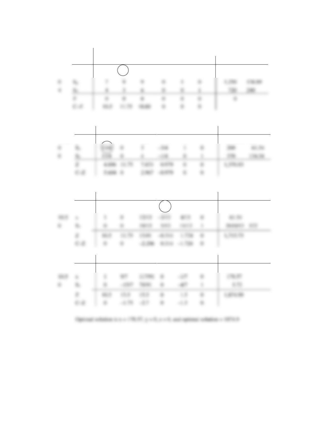
2.
a.
Minimize Z =
21x1
+ 18x2
s.t.
5x1
+ 10x2
+ A1– S1
= 100
2x1
+ 1x2
+ A2 – S2
= 10
C
21
18
M
0
M
0
C
21
18
M
0
M
0
II.
C
Var
x1
x2
A1
S1
A2
S2
bi
ratio
18
x2
0.5
1
0.1
–0.1
0
0
10
20
Z
[1.5M+9]
18
180
0
C
21
18
0
0
III.
C
Var
x1
x2
S1
S2
bi
18
x2
0
1
–0.1333
0.333
10
Z
21
18
–0.99999
–8.000
180
0
0
0.99999
8.000
The optimal solution: x1 = 0; x2 = 10; Z = 180
C
M
2
1
0
0
1
10
Z
7M
11M
110M
Chapter 19 – Linear Programming
19–34
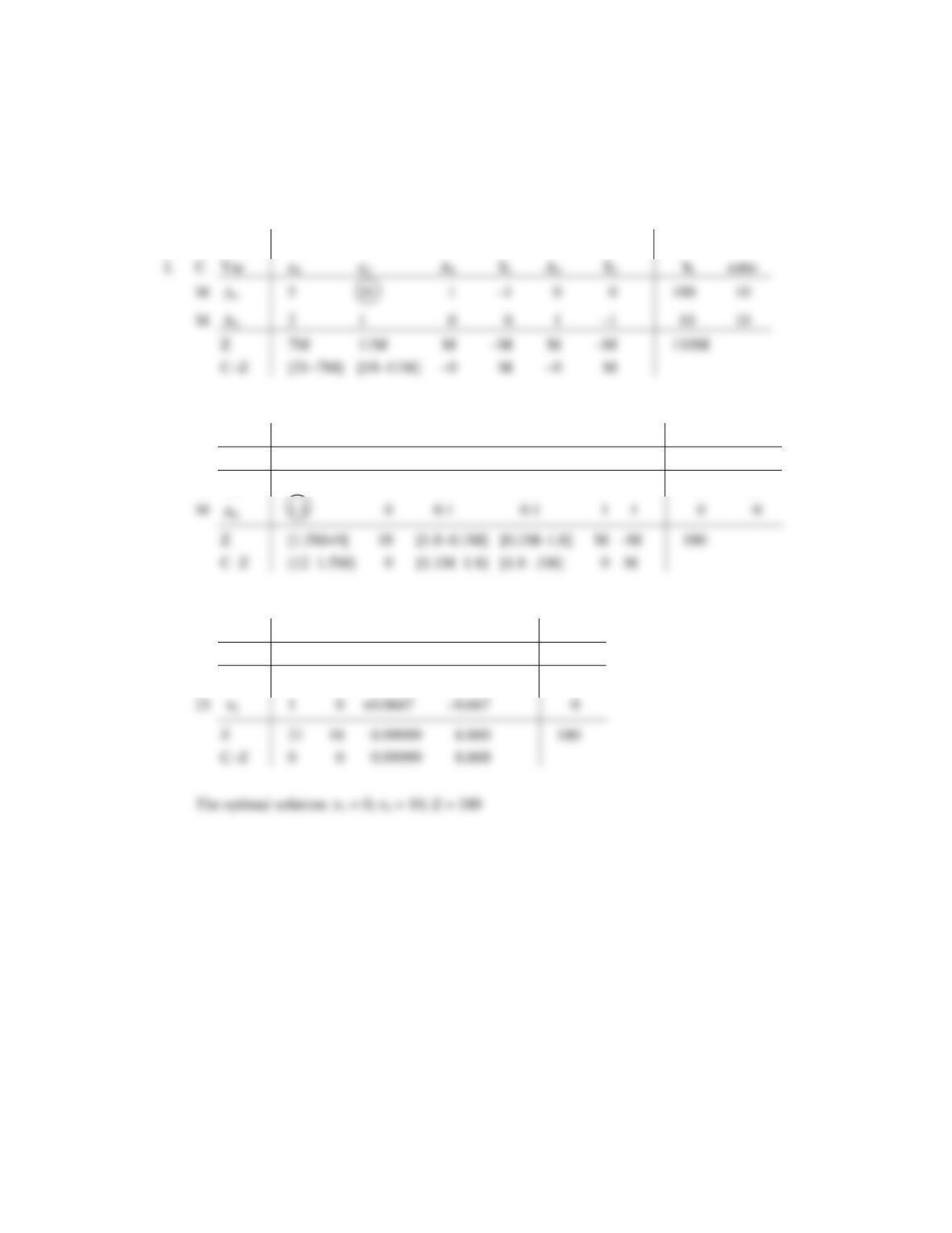
Solutions (continued)
2.
b.
I.
C
2
5
3
M
0
M
0
M
0
Var
x
y
z
A1
S1
A2
S2
A3
S3
bi
M
A1
16
10
18
1
–1
0
0
0
0
340
M
A2
11
12
13
0
0
1
–1
0
0
300
M
A3
2
6
5
0
0
0
0
+1
–1
120
Z
29M
28M
36M
M
–M
M
–M
M
–M
760M
C–Z
[–29M+2]
[–28M+5]
[–36M+3]
0
M
0
M
0
M
III.
C
Var
x
y
z
S1
A2
S2
S3
bi
3
z
1.31
0
1
–.1034
0
0
.1724
14.48
M
A2
3.069*
0
0
.3103
1
–1
1.483
16.55
5
Y
–0.7586
1
0
0.08621
0
0
–0.3103
7.931
Z
[3M+.138]
5
3
[.3M+.121]
–M
[1.5M–1.03]
[16.55M+83.1]
C–Z
[–3.1M+1.86]
0
0
[–.3M–.121]
0
M
[–1.5M+1.03]
IV.
C
Var
x
y
z
S2
S3
bi
3
z
0
0
1
.427
2
x
1
0
0
.4831
5.393
5
y
0
1
0
.05618
12.02
Z
C–Z
0
0
0
0.6067
0.1348
V.
C
Var
x
y
z
S1
S2
S3
bi
3
z
2.333
0
1
0
–0.3333
.6667
20
0
S1
9.889
0
0
1
–3.222
4.778
53.33
5
y
1
0
0
3.333
Z
C–Z
3.056
0
0
0
–0.3889
1.6111
II.
C
Var
x
y
z
S1
A2
S2
A3
S3
bi
3
Z
1
–.0556
0
0
0
0
M
A2
–.5556
4.778
0
.722
1
0
0
54.44
M
A3
3.222*
0
.2778
0
0
1
–1
25.56
Z
M
–M
M
–M
80M+56.7
C–Z
[+3M+.7]
[–8M+3.3]
0
[2M–47]
[–M+.17]
0
M
0
M
Chapter 19 – Linear Programming
19–35
Solutions (continued)
VI.
C
Var
x
y
z
S1
S2
S3
bi
3
z
.4
1.2
1
0
0
–0.200
24
0
S1
–8.8
11.6
0
1
0
–3.6
92
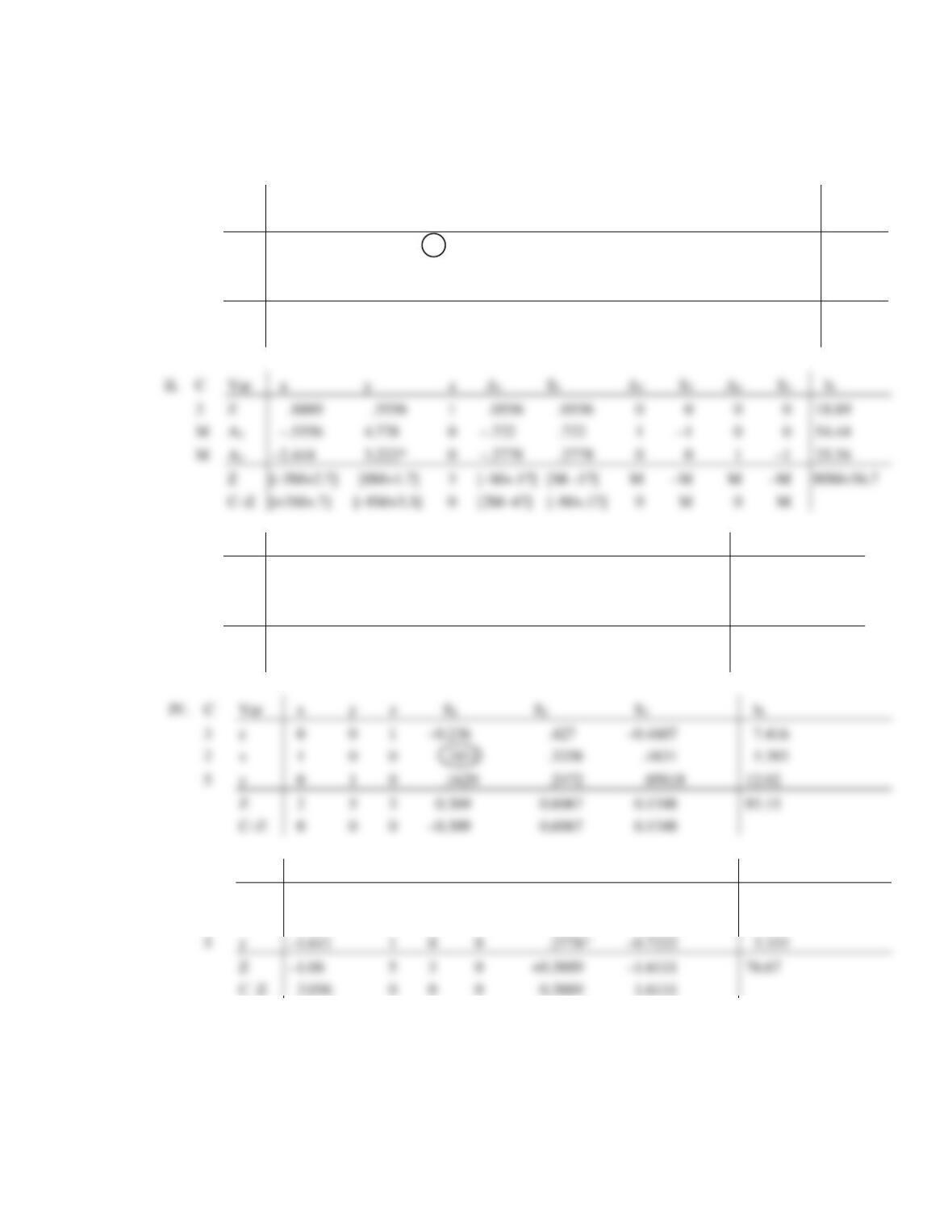
3.
C
3
4
8
0
0
M
M
Var
x1
x2
x3
S1
S2
A1
A2
bi
bi/aij
M
A1
2
1
0
–1
0
1
0
6
6/2 = 3
M
A2
0
1
2
0
–1
0
1
4
–
Zj
2M
2M
2M
–M
–M
M
M
10M
Cj–Zj
3–2M
4–2M
8–2M
M
M
0
0
C
3
4
8
0
0
Var
x1
x2
x3
S1
S2
bi
bi/aij
3
x1
1
½
0
–½
0
3
3 ½ = 6
M
A2
0
1
2
0
–1
4
Zj
3
2M
–3/2
–M
4M+9
Cj–Zj
0
5/2 –M
8–2M
3/2
M
C
3
4
8
0
0
Var
x1
x2
x3
S1
S2
bi
bi/aij
3
x1
1
½
0
–½
0
3
3 ½ = 6
8
x3
0
½
1
0
–½
2
2 ½ = 4
Zj
3
11/2
8
–3/2
–4
25
Cj–Zj
0
–3/2
0
3/2
4
C
3
4
8
0
0
Var
x1
x2
x3
S1
S2
bi
3
1
0
1
4
x2
0
1
2
0
4
3
4
5
19
Cj–Zj
0
0
3
3/2
5/2
.8
1.4
0
0
0
.6
Optimal solution is: x = 0; y = 0; z = 24 and Z = 72.0
Chapter 19 – Linear Programming
19–36
Solutions (continued)
4.
Cj
8
2
0
0
Var
x1
x2
S1
S2
bi
0
S1
4
5
1
0
20
0
S2
2
6
0
1
18
Zj
0
0
0
0
0
Cj–Zj
8
2
0
0
Cj
Var
x1
x2
S1
S2
bi
8
1
5/4
0
0
S2
0
7/2
1
Zj
8
2
0
Cj–Zj
0
0