
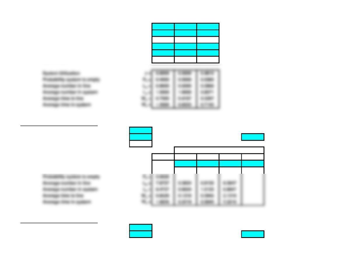
Multiple Priorities Waiting Line Model
<Back
Service rate m = 1
Increment Dm = 1 Number of servers M = 6
Service time 1/m = 1.0000
Class
System 1 2 3 4
Arrival rate l = 5.0000 2 2 1
System Utilization r = 0.8333
Probability system is empty P0 = 0.0045
60%
80%
100%
1.5
2
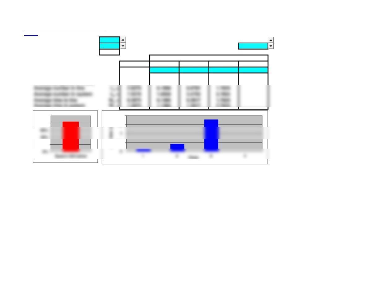
Average number in line Lq = 2.9376 0.2938 0.8813 1.7625
Average number in system Ls = 7.9376 2.2938 2.8813 2.7625
Average time in line Wq = 0.5875 0.1469 0.4406 1.7625
Calculations:
lamda = 5
mu = 1
M P0
26.000 -8.333 -0.429
318.500 -31.250 -0.078
439.333 -104.167 -0.015
565.375 #DIV/0! #DIV/0!
691.417 130.208 0.005
8128.619 25.835 0.006
10 143.689 5.382 0.007
12 147.604 0.874 0.007
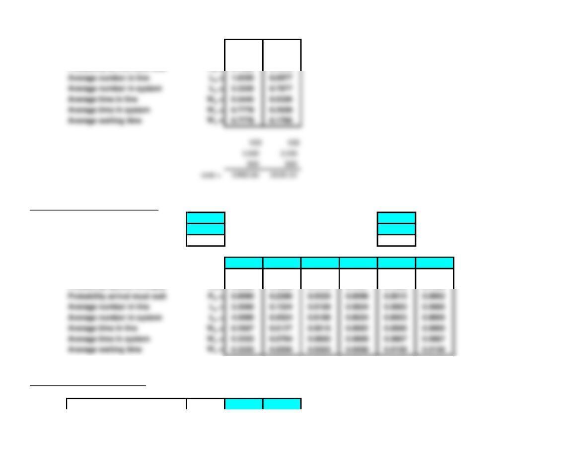
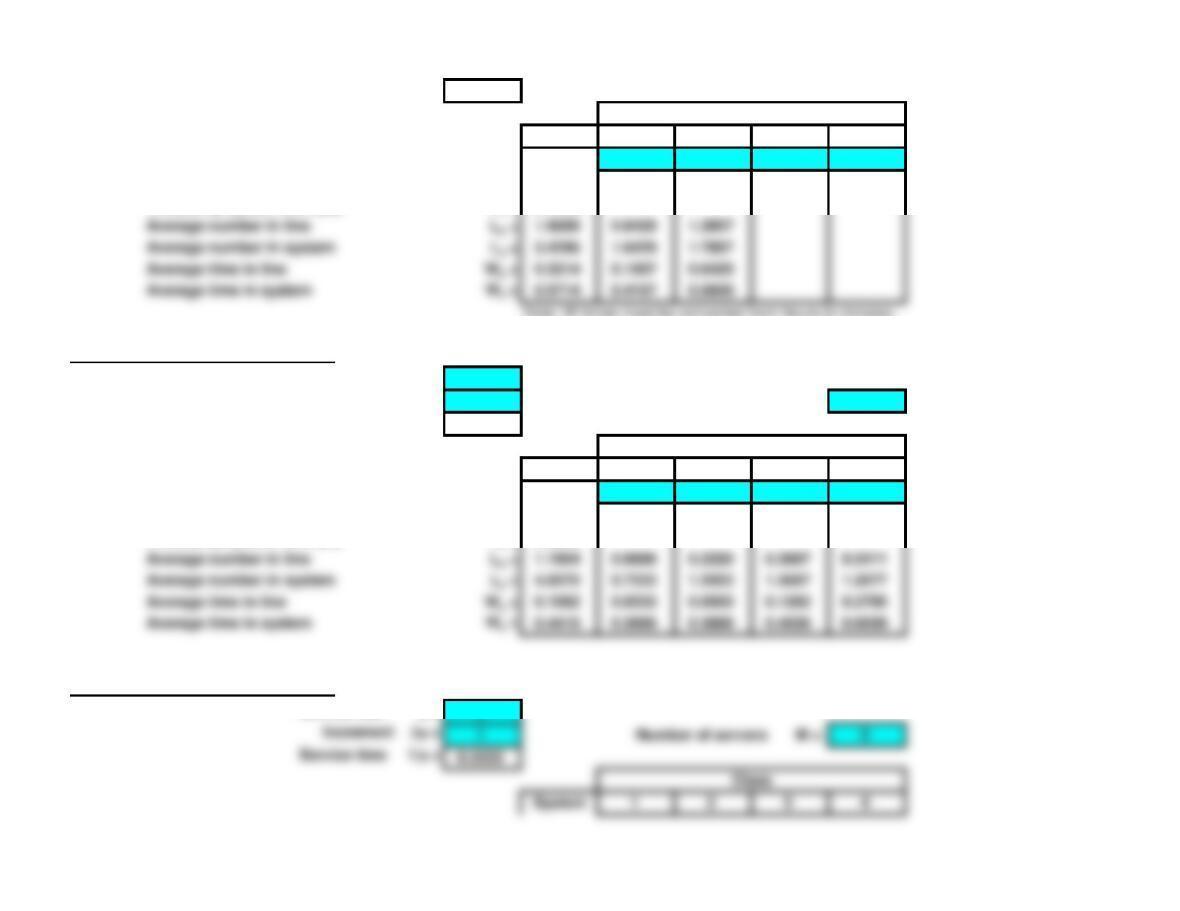
Multiple Priorities Waiting Line Model
<Back
Service rate m = 1
Increment Dm = 1 Number of servers M = 6
Service time 1/m = 1.0000
Class
System 1 2 3 4
Arrival rate l = 5.0000 1.5 2.5 1
System Utilization r = 0.8333
Probability system is empty P0 = 0.0045
Average time in system Ws = 1.5875 1.1306 1.3917 2.7625
20%
80%
100%
0.5
1.5
2
Ave. time in line
Average number in line Lq = 2.9376 0.1958 0.9792 1.7625
Average number in system Ls = 7.9376 1.6958 3.4792 2.7625
Average time in line Wq = 0.5875 0.1306 0.3917 1.7625
Calculations:
lamda = 5
mu = 1
M P0
11.000 -1.250 -4.000
318.500 -31.250 -0.078
439.333 -104.167 -0.015
565.375 #DIV/0! #DIV/0!
7113.118 54.253 0.006
9138.307 12.110 0.007
11 146.381 2.243 0.007
12 147.604 0.874 0.007
Finite Source Waiting Line Model
<Back
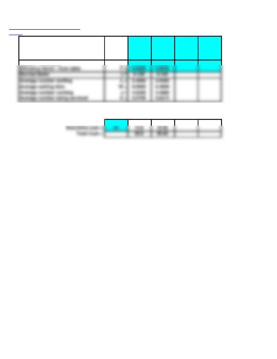
Population Size N = 5 5
Number of servers M = 1 2
Average service time T = 10 10
Average time between service calls U = 70 70
P(wait) – from table D = 0.5750 0.0820
Per Time
Unit
Service cost = 10 10 20
Note: You must enter D and F (based on N, c, and M) from the table in the text.
Efficiency factor – from table F = 0.9200 0.9940
Average number waiting L = 0.4000 0.0300
Average waiting time W = 6.9565 0.4829
Average number running J = 4.0250 4.3488
Average number being serviced H = 0.5750 0.6213
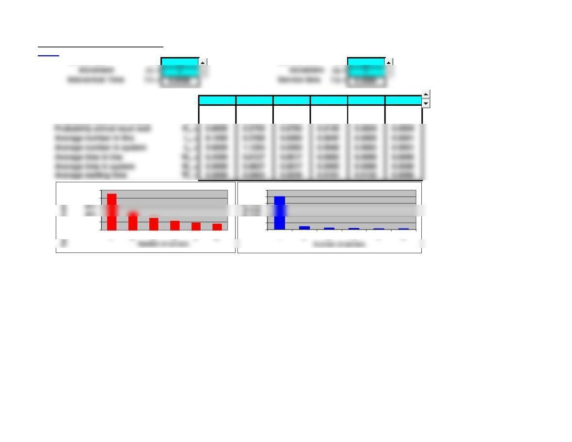
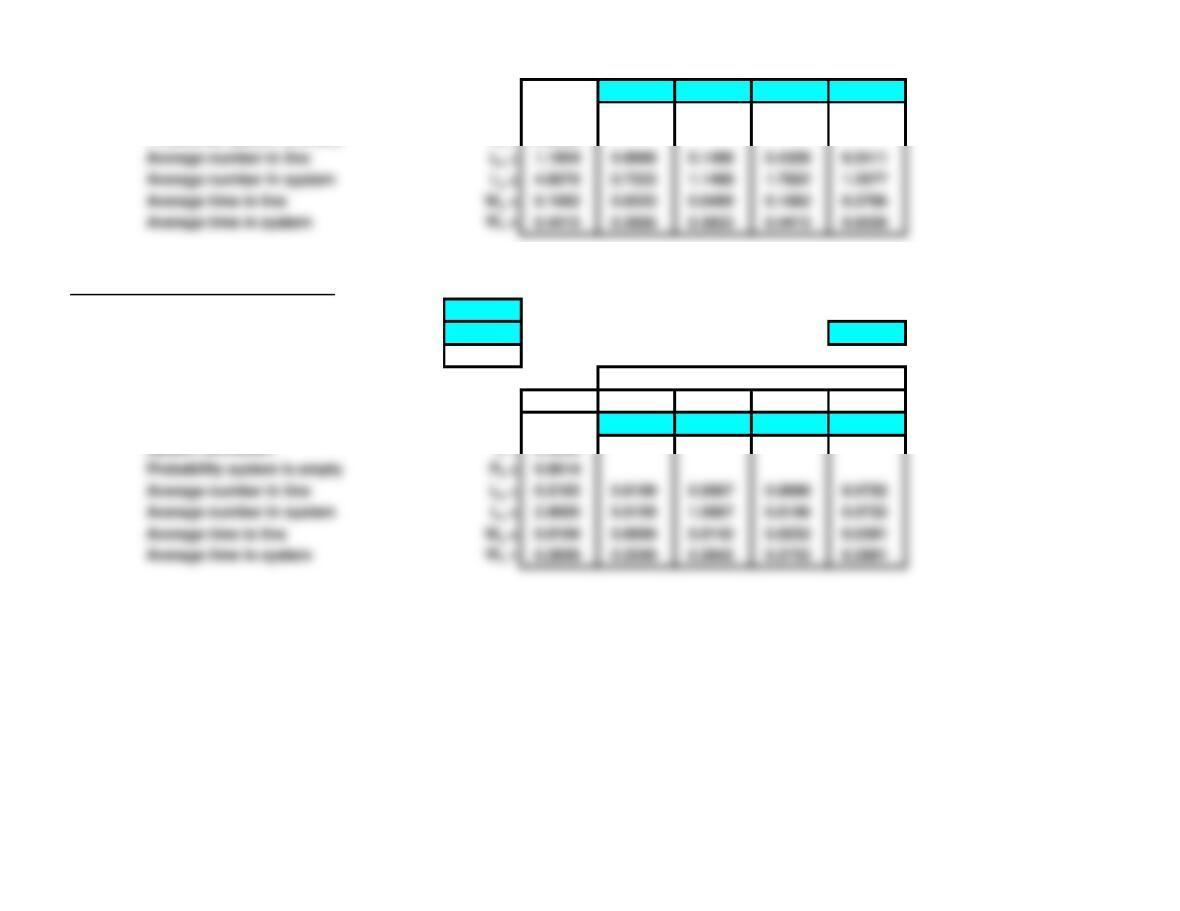
Multiple Channel Waiting Line Model
<Back
Arrival rate l = 18 Service rate m = 20
Number of servers (max 12) M = 1 2 3 4 5 6
System Utilization r = 0.9000 0.4500 0.3000 0.2250 0.1800 0.1500
Probability system is empty P0 = 0.1000 0.3793 0.4035 0.4062 0.4065 0.4066
Probability arrival must wait Pw = 0.9000 0.2793 0.0700 0.0143 0.0024 0.0004
Average number in line Lq = 8.1000 0.2285 0.0300 0.0042 0.0005 0.0001
Average number in system Ls = 9.0000 1.1285 0.9300 0.9042 0.9005 0.9001
Average time in line Wq = 0.4500 0.0127 0.0017 0.0002 0.0000 0.0000
Average time in system Ws = 0.5000 0.0627 0.0517 0.0502 0.0500 0.0500
0%
20%
80%
100%
0.00
0.10
0.20
0.50
0.60
1 2 3 4 5 6
Waiting Time
Interarrival Time 1/l = 0.0556 Service time 1/m = 0.0500
Calculations:
l = 18
m = 20
M P0
11.000 9.000 0.100
32.305 0.174 0.403
52.454 0.006 0.407
72.459 0.000 0.407
92.460 0.000 0.407
11 2.460 0.000 0.407
12 2.460 0.000 0.407
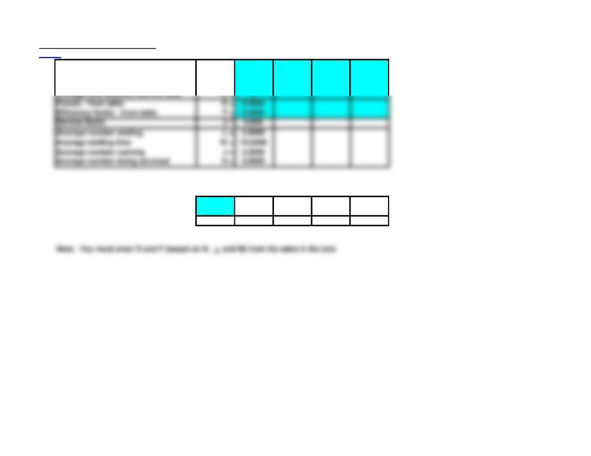
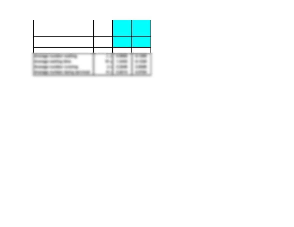
Finite Source Waiting Line Model
<Back
Population Size N = 10
Number of servers M = 3
Average service time T = 9
Average time between service calls U = 6
Per Time
Unit
Service cost =
Downtime cost =
Total Cost =
P(wait) – from table D = 0.9960
Efficiency factor – from table F = 0.5000
Average number waiting L = 5.0000
Average waiting time W = 15.0000
Average number running J = 2.0000
Average number being serviced H = 3.0000
Chapter 18 – Problems 1-9 Note: This worksheet displays results only, you must copy the shaded
<Back area into the corresponding template to make additional calculations.
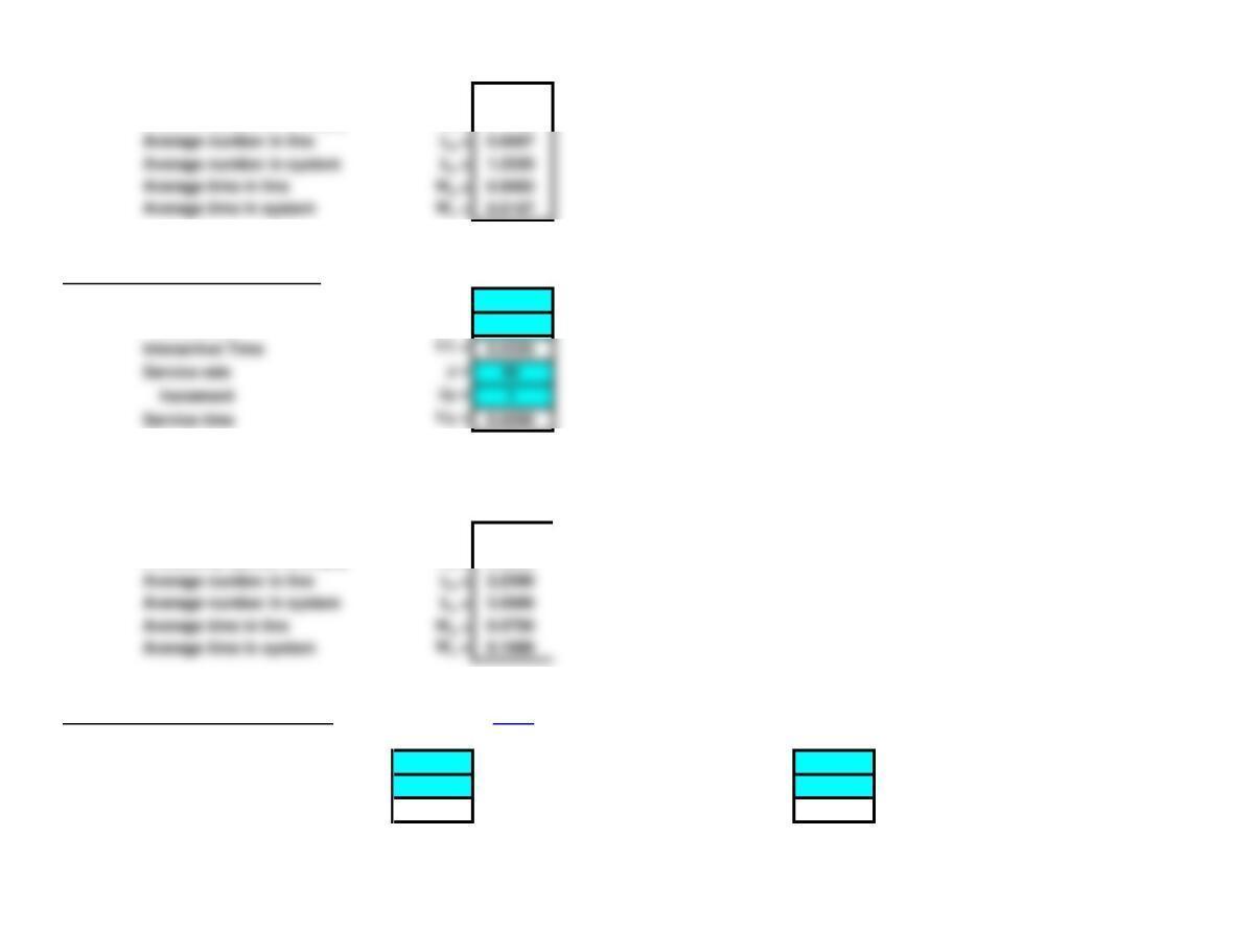
1. Single Channel Waiting Line Model
Arrival rate
l = 3
Increment
Dl = 1
Interarrival Time
1/l = 0.3333
Exponential
Service
Time
System Utilization
r = 0.7500
Probability system is empty
P0 = 0.2500
2. Single Channel Waiting Line Model
Arrival rate
l = 80
Increment
Dl = 1
1/l = 0.0125
Dm = 1
1/m = 0.0083
Dm = 1
1/m = 0.2500
System Utilization
r = 0.6667
Probability system is empty
P0 = 0.3333
3. Single Channel Waiting Line Model
Arrival rate
l = 30
Increment
Dl = 1
Dm = 1
Exponential
Service
Time
System Utilization
r = 0.7500
Probability system is empty
P0 = 0.2500
4. Multiple Channel Waiting Line Model Basic
Arrival rate l = 0.45 Service rate m = 0.5
Increment Dl = 0.1 Increment Dm = 0.1
Interarrival Time 1/l = 2.2222 Service time 1/m = 2.0000
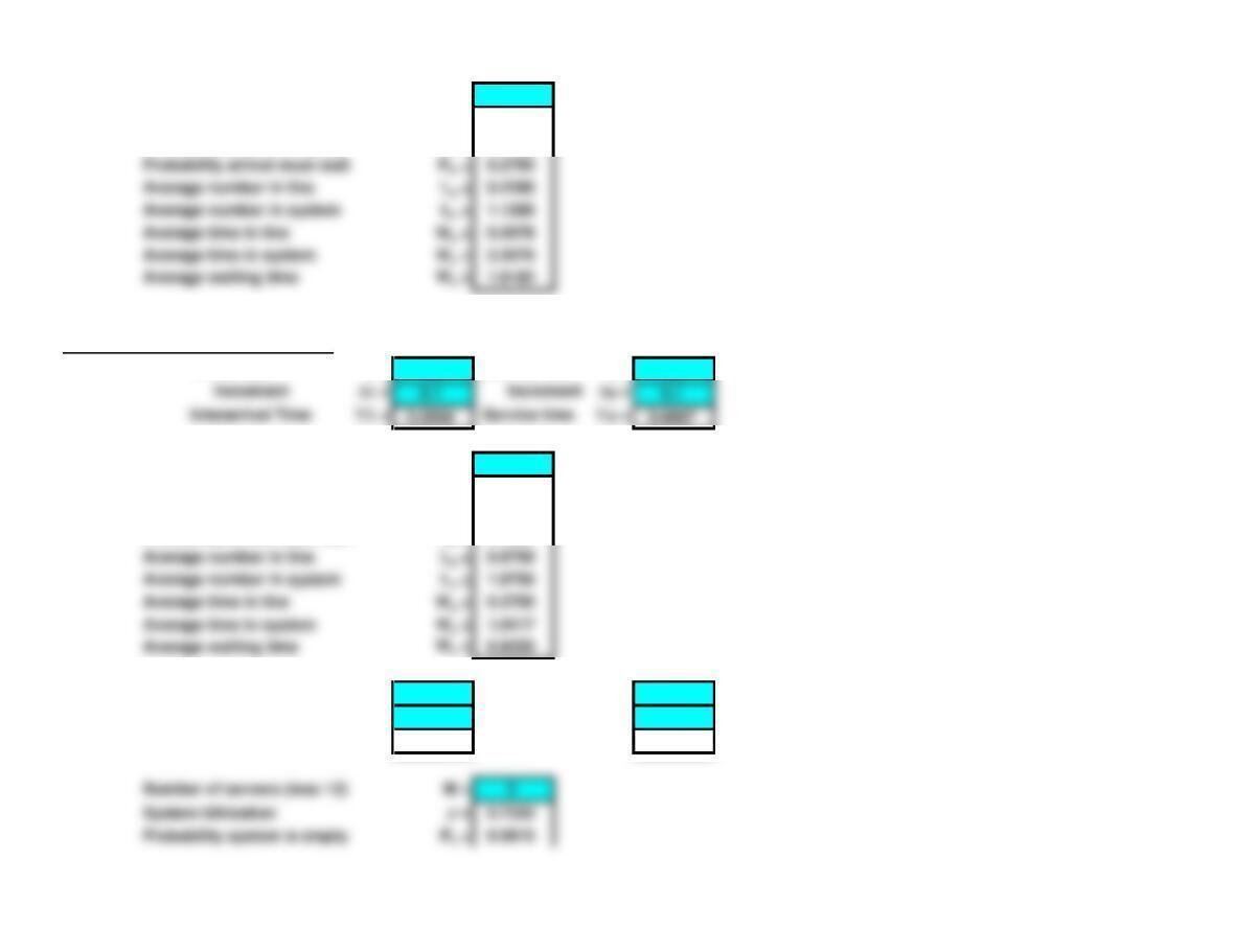
Number of servers (max 12) M = 2
System Utilization
r = 0.4500
Probability system is empty
P0 = 0.3793
5. Multiple Channel Waiting Line Model
Arrival rate l = 1.8 Service rate m = 1.5
Increment Dl = 0.1 Increment Dm = 0.1
Interarrival Time 1/l = 0.5556 Service time 1/m = 0.6667
Number of servers (max 12) M = 2
System Utilization
r = 0.6000
Probability system is empty
P0 = 0.2500
Probability arrival must wait
Pw = 0.4500
Arrival rate l = 2.2 Service rate m = 1
Increment Dl = 0.1 Increment Dm = 0.1
Interarrival Time 1/l = 0.4545 Service time 1/m = 1.0000
P0 = 0.0815
Pw = 0.2793
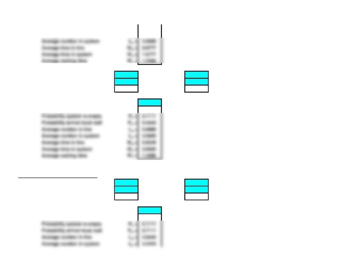
Probability arrival must wait
Pw = 0.5422
Average number in line
Lq = 1.4909
Arrival rate l = 1.4 Service rate m = 0.7
Increment Dl = 0.1 Increment Dm = 0.1
Interarrival Time 1/l = 0.7143 Service time 1/m = 1.4286
Number of servers (max 12) M = 3
System Utilization
r = 0.6667
Pw = 0.4444
Lq = 0.8889
Ls = 2.8889
6. Multiple Channel Waiting Line Model
Arrival rate l = 40 Service rate m = 25
Increment Dl = 0.1 Increment Dm = 0.1
Interarrival Time 1/l = 0.0250 Service time 1/m = 0.0400
Number of servers (max 12) M = 2
System Utilization
r = 0.8000
Ls = 3.6909
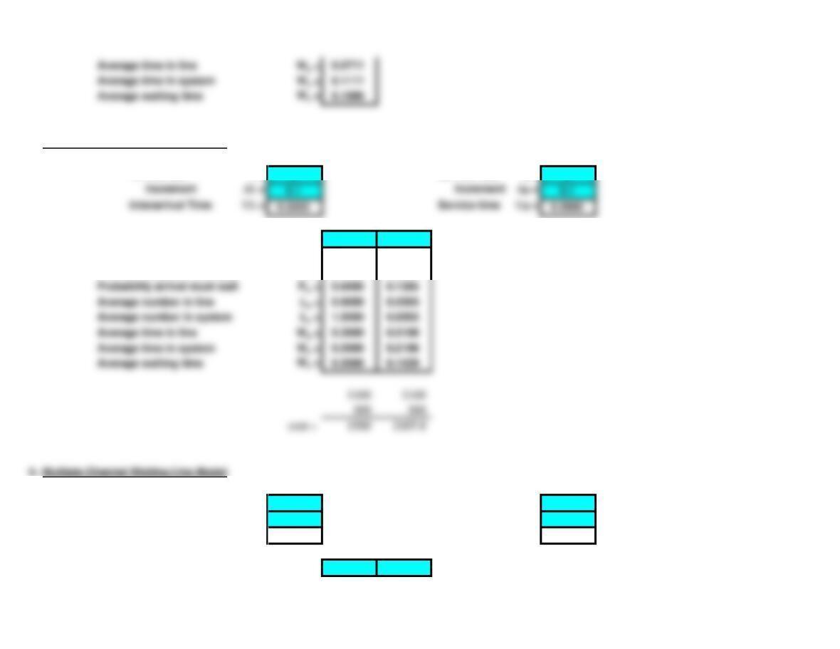
7a. Multiple Channel Waiting Line Model
Arrival rate l = 3Service rate m = 5
Increment Dl = 0.1 Increment Dm = 0.1
Interarrival Time 1/l = 0.3333 Service time 1/m = 0.2000
Number of servers (max 12) M = 1 2
System Utilization
r = 0.6000 0.3000
Probability system is empty
P0 = 0.4000 0.5385
Arrival rate l = 3Service rate m = 4.2856
Increment Dl = 0.1 Increment Dm = 0.1
Interarrival Time 1/l = 0.3333 Service time 1/m = 0.2333
Number of servers (max 12) M = 1 2
System Utilization
r = 0.7000 0.3500
Probability system is empty
P0 = 0.3000 0.4815
Probability arrival must wait
Pw = 0.7000 0.1815
8. Multiple Channel Waiting Line Model
Arrival rate l = 12 Service rate m = 15
Increment Dl = 0.1 Increment Dm = 0.1
Interarrival Time 1/l = 0.0833 Service time 1/m = 0.0667
Number of servers (max 12) M = 1 2 3 4 5 6
System Utilization
r = 0.8000 0.4000 0.2667 0.2000 0.1600 0.1333
Probability system is empty
P0 = 0.2000 0.4286 0.4472 0.4491 0.4493 0.4493
Pw = 0.8000 0.2286 0.0520 0.0096 0.0015 0.0002
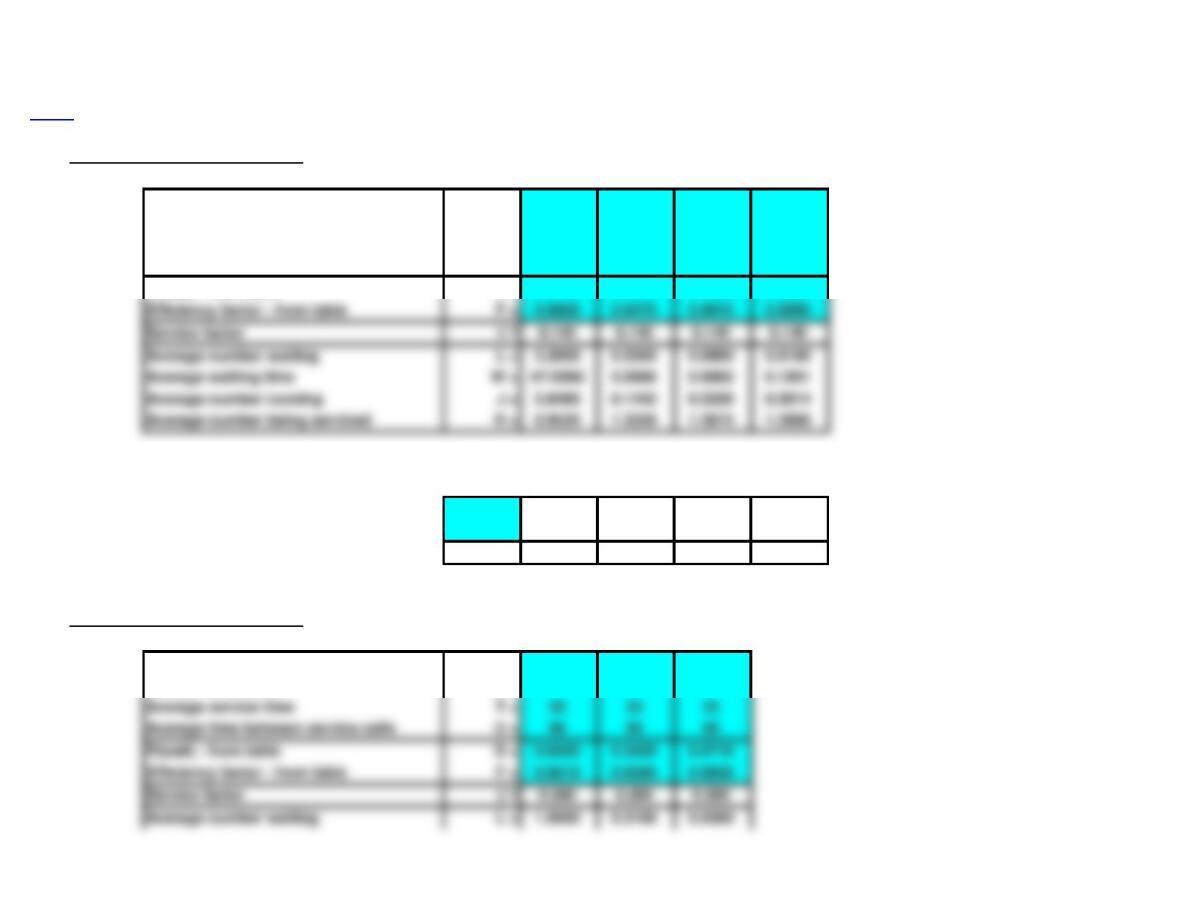
9. Finite Source Waiting Line Model
Population Size N = 5 5
Number of servers M = 1 2
Average service time T = 1 1
Average time between service calls
U = 4 4
P(wait) – from table D = 0.6890 0.1940
Efficiency factor – from table F = 0.8010 0.9760
Service factor
c = 0.200 0.200
Chapter 18 – Problems 10-17 Note: This worksheet displays results only, you must copy the shaded
<Back area into the corresponding template to make additional calculations.
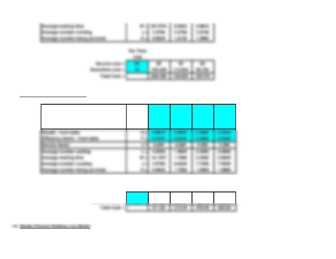
10. Finite Source Waiting Line Model
Population Size N = 10 10 10 10
Number of servers M = 1 2 3 4
Average service time T = 14 14 14 14
Average time between service calls U = 86 86 86 86
P(wait) – from table D = 0.9190 0.4370 0.1320 0.0280
Per Time
Unit
Service cost = 15 15 30 45 60
Downtime cost = 70 290.64 129.906 103.418 98.602
Total Cost = 305.64 159.906 148.418 158.602
11. Finite Source Waiting Line Model
Population Size N = 5 5 5
Number of servers M = 1 2 3
12. Finite Source Waiting Line Model
Population Size N = 10 10 10 10
Number of servers M = 1 2 3 4
Average service time T = 2 2 2 2
Average time between service calls U = 8 8 8 8
Per Time
Unit
Service cost = 30 30 60 90 120
Downtime cost = 80 481.92 253.44 180.48 163.84
Arrival rate
l = 1.2 1.2 1.2
Increment
Dl = 1 1 1
Interarrival Time
1/l = 0.8333 0.8333 0.8333
Service rate
m = 22.4 2.6
Increment
Dm = 10.1 0.1
Service time
1/m = 0.5000 0.4167 0.3846
14. Multiple Priorities Waiting Line Model
Service rate m = 5
Increment Dm = 1 Number of servers M = 2
Service time 1/m = 0.2000
Class
System 1 2 3 4
Arrival rate
l = 9.0000 333
System Utilization
r = 0.9000
15. Multiple Priorities Waiting Line Model
Service rate m = 4
Increment Dm = 1 Number of servers M = 2
r = 0.6000 0.5000 0.4615
Service time 1/m = 0.2500
Class
System 1 2 3 4
Arrival rate
l = 6.0000 4 2
System Utilization
r = 0.7500
Probability system is empty
P0 = 0.1429
Note: W times must be converted from hours to minutes.
16. Multiple Priorities Waiting Line Model
Service rate m = 3
Increment Dm = 1 Number of servers M = 5
Service time 1/m = 0.3333
Class
System 1 2 3 4
Arrival rate
l = 11.0000 2432
System Utilization
r = 0.7333
Probability system is empty
P0 = 0.0209
16c. Multiple Priorities Waiting Line Model
Service rate m = 3
Increment Dm = 1 Number of servers M = 5
Arrival rate
l = 11.0000 2342
System Utilization
r = 0.7333
Probability system is empty
P0 = 0.0209
17. Multiple Priorities Waiting Line Model
Service rate m = 4
Increment Dm = 1 Number of servers M = 5
Service time 1/m = 0.2500
Class
System 1 2 3 4
Arrival rate
l = 11.0000 2432
System Utilization
r = 0.5500