Chapter 18 – Management of Waiting Lines
18-1
CHAPTER 18
MANAGEMENT OF WAITING LINES
Teaching Notes
Some of the math and calculations can be left out in order to focus more clearly on the concepts of
waiting lines. For example, all infinite source problems, including single channel (except constant service
time) can be handled using the infinite source queuing table. In the past, queuing presented students with
a good bit of computational requirements, and because of that, students frequently lost sight of the
underlying concepts. With less emphasis on math of calculations, students can handle individual problems
Answers to Discussion and Review Questions
2. Variations in service and/or arrival rates create instances in which demand temporarily exceeds
capacity.
3. Commonly used measures of system performance include the average number waiting and
5. Supermarkets advertise specials early in the week in an attempt to attract customers on slower
6. An infinite source model applies when system entry is unrestricted, or when the potential number
7. The multiple priority approach is appropriate whenever the cost or criticalness of waiting for
service differs significantly for different customer (categories).
8. Among the possibilities: meet your neighbors, keep you from wandering around, eliminate line
9. As the utilization increases, the expected length of the waiting line increases. At some point,
Chapter 18 – Management of Waiting Lines
18-2
Taking Stock
1. In waiting line decisions, the primary trade-off is the cost of having too many employees (cost of
service or idle time) vs. cost of not having enough employees (cost of waiting). If the company
2. In assessing the cost of customer waiting for service involving the general public, the customers
themselves, marketing, finance and operations managers or representatives from those
3. The technology has had a profound impact on analyzing waiting line systems. First of all, through
the use of computers and simulation studies, we have been able to quickly analyze the impact of
different levels of employment on waiting lines. The sophisticated computer systems have been
able to perform what-if analysis and rapidly show the simulated results with different arrival rates
and service times.
Critical Thinking
1. Financial and space constraints may limit management options. Psychological options may be
2. a. (Varied answers.)
b. With a service rate of 10/hr., Lq = 3.200
With a service rate of 20/hr., Lq = 0.267
3. Relevant factors include the travel distance in terms of time and cost in a centralized location vs.
Chapter 18 – Management of Waiting Lines
18-3
4. Mass customization involves providing standardized services or goods, while incorporating some
degree of customization. Mass customization may be applied at the Eat Now restaurant by
streamlining and standardizing the operations such that it becomes more efficient and faster to
serve the customers while trying to maintain as many of the menu options as possible. However,
there is a trade-off between standardizing the services and maintaining the menu options. The
5. Student answers will vary.
Memo Writing Exercises
1. The advantage of having a centralized tool crib is that all the tools can be stored at a central,
single location, making it easier to control the tool inventory. The single location will most likely
2. Multiple priority rule would be used when the First-Come-First-Served (FCFS) rule is
inappropriate. For example, in production scheduling, Earliest Due Date (EDD) rule is generally
more appropriate than FCFS rule. In computer processing of jobs, Shortest Processing (SPT)
Chapter 18 – Management of Waiting Lines
18-4
Solutions
1. [Infinite source, single channel]
= 3/day
,75.r =
=
M = 1. From table 18–4, Lq = 2.25 customers
2. [Infinite source, single channel, constant service]
= 80 customers/hrs.
= 120 customers/hr.
3. = 30/hr. Single Channel
= 40/hr.
minutes 5.4.hrs 075.
30
25.2
L
Wq
q==+
=
WS = Wq +1/ = 4.5 + 1.5 = 6 minutes
Chapter 18 – Management of Waiting Lines
18-5
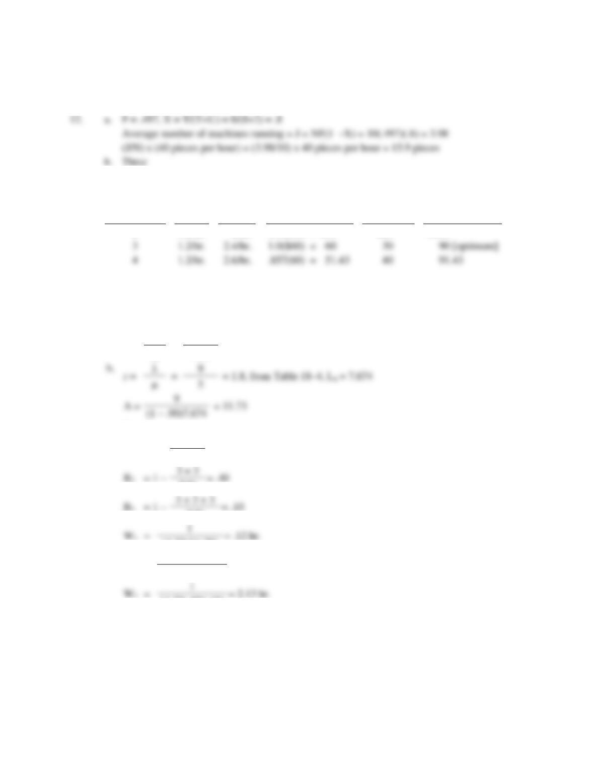
4. [Infinite source, multiple channel]
b.
.80.
45.===
r
From infinite queuing table with M = 2, Lq = .229
d.
28.
818.1
509.===
a
q
wW
W
P
where
1.818
.45. – 2(.50)
11 ==
−
=
Mu
Wa
5. a.
Period
M
r = /
Lq
Wq =
Lq
Pw
morning
1.8/min.
1.5/min.
2
1.2
.675
.375
.450
evening
1.4/min.
3
2.0
.889
.635
.444
Afternoon
.101
.733
Chapter 18 – Management of Waiting Lines
18-6
6.
= 40 trucks/hr.
a.
,6.1=
Lq = 2.844 from Table 18–4
= 4.444 trucks
It would grow increasingly long.
)PP(1P
or
7111.
10.
W
P
0711.
40
W
10W
a
q
W
q
q
+−=
===
==
=
2.844 (1 – .80)
n =
ln k
= 13.186
lnρ
7. a.
= 3 trucks/day
Truck + Driver cost = $300/day
= 5 trucks/day
Dock + Loading crew = $1,100/day
M = ?
1.5
1.5($300) = $450.00
$1,550.00*
.659($300) = 197.70
M = 2
Chapter 18 – Management of Waiting Lines
18-7
b.
= 3 trucks/day
Truck + Driver cost = $300/day
= 6 trucks/day
Dock + Loading crew + equip.= $1,200/day
M = ?
8.
= 12/hr. [1/5 min. x 60 min./hr. = 12/hr.]
= 15/hr.
M = 2 clerks
Po = .429
= .152 + .80 = .952
b.
228.
05556.
01267.
W
W
P
a
q
w===
2(15) – 12
2(15)
$M
$20
3.2 + .8 = 4
.152 + .8 = .952
68.56
1
1
9.
N = 5
T = 1 day
X =
T
=
1
= .20
U = 4 days
T + U
1 + 4
From finite queuing table, with M = 1, N = 5 and X = .20, D = 0.801
and F = .801
a. L = N(1 – F) = 5(1 – .801) = .995 customers
M($1,200)
[opt.]
1.0($300) = $300.00
$1,500.00*
.533
.533($300) = 159.90
2,400
Chapter 18 – Management of Waiting Lines
18-8
10.
N = 10
T = 14 minutes
U = 86 minutes
X =
T
=
14
= .14
M = 2 operators
T + U
14 + 86
and F = .947
8.144
N
10
From finite queuing table, with N = 10, X = .14 and M = 2, D = .437
J = NF(1 – X) = 10(.947)(.86) = 8.144
M
Total Cost
.680
4.152(70) = $290.64
.947
1.856(70) = 129.92
159.92
[opt.]
.991
1.477(70) = 103.39
148.39*
.999
1.409(70) = 98.63
158.63
11.
N = 5
M = 1
X =
T
=
35
= .28
T = 35 minutes
T + U
35 + 90
U = 90 minutes
From finite queuing table, with N = 5, X = .28 and M = 1, D = .842
and F = .661.
(60) =
2.3796
(60) = 28.56 p/hr.
b.
M
F
J = NF(1–X)
Machine Cost
(N–J)$70
Operating
Cost
Total Cost
1
.661
2.380
2.62($70) = 183.42
$20
$203.42
[opt]
3.377
1.623($70) = 113.62
3.575
1.425($70) = 99.76
W + T =
L(T + U)
+ T =
+ 1 = 2.24 days
5 – .995
Chapter 18 – Management of Waiting Lines
18-9
13.
[Infinite source, single channel]
[truck cost]
No. of crew
members
Ls ($60/hr.)
Crew Cost
Total Cost
2
1.2/hr.
2/hr.
1.5($60) = $90
$20
$110
3
1.2/hr.
2.4/hr.
1.0($60) = 60
90 [optimum]
4
1.2/hr.
2.6/hr.
.857(60) = 51.43
91.43
14.
1 = 3/hr.
= 5/hr.
2 = 3/hr.
M = 2 servers
3 = 3/hr.
a.
=
=
9
= .90, or 90%
s
2(5)
b.
9
5
A =
= 11.73
(1 – .90)7.674
Bo = 1
B1 = 1 –
3
= .70
2(5)
= .40
2(5)
B3 = 1 –
3 + 3 + 3
= .10
2(5)
= .12 hr.
11.73(1)(.70)
W2 =
1
= .3045 hr.
11.73(.70)(.40)
= 2.13 hr.
11.73(.40)(.10)
c. L1 = 3(.12) = .36
L2 = 3(.3045) = .91
L3 = 3(2.13) = 6.39
Chapter 18 – Management of Waiting Lines
18–10
15.
1 = 4/hr
= 4/ hr.
r =
/2
= 6/8 = .75
2 = 2/hr
M = 2
= 4/hr.
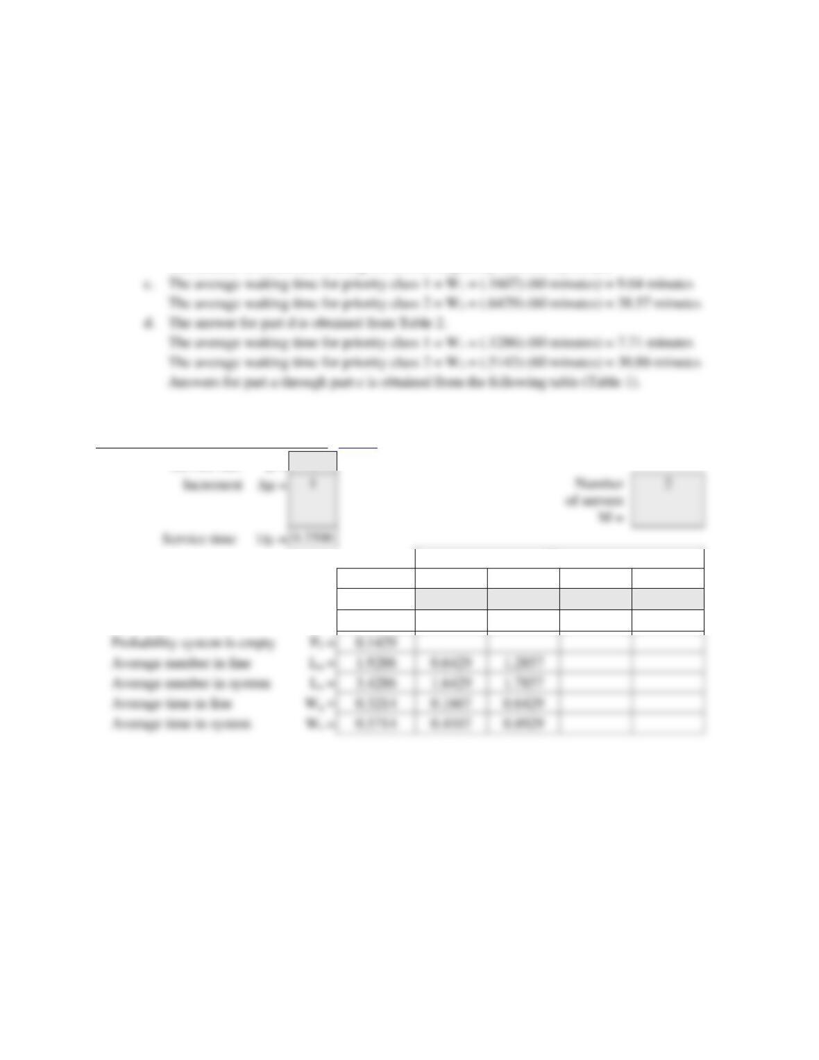
Using the Excel spreadsheets for the multiple priorities waiting line model, we obtain the
following table of output. Based on this table of output
a. the system utilization = = .75
b. The number of customers waiting for service in priority class 1 = L1 = .643
The number of customers waiting for service in priority class 2 = L2 =1.286
Table 1
Multiple Priorities Waiting Line Model
<Back
Service rate =
4
Class
System
1
2
3
4
Arrival rate
=
6.0000
4
2
System Utilization
=
0.7500
Probability system is empty
Average number in line
Average number in system
Average time in line
Average time in system
Chapter 18 – Management of Waiting Lines
18–11
d. Table 2
Multiple Priorities Waiting Line Model
<Back
Service rate =
4
Class
System
1
2
3
4
Arrival rate
=
6.0000
3
3
System Utilization
=
0.7500
Probability system is empty
P0 =
0.1429
Average number in line
1.9286
Average number in system
Ls =
3.4286
Average time in line
0.3214
Average time in system
0.5714
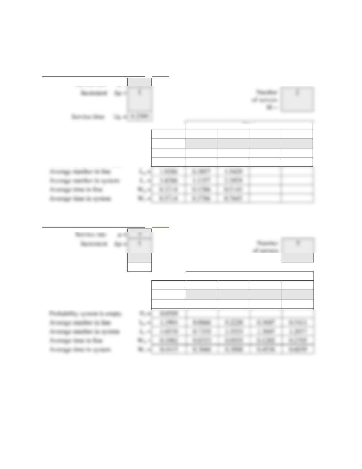
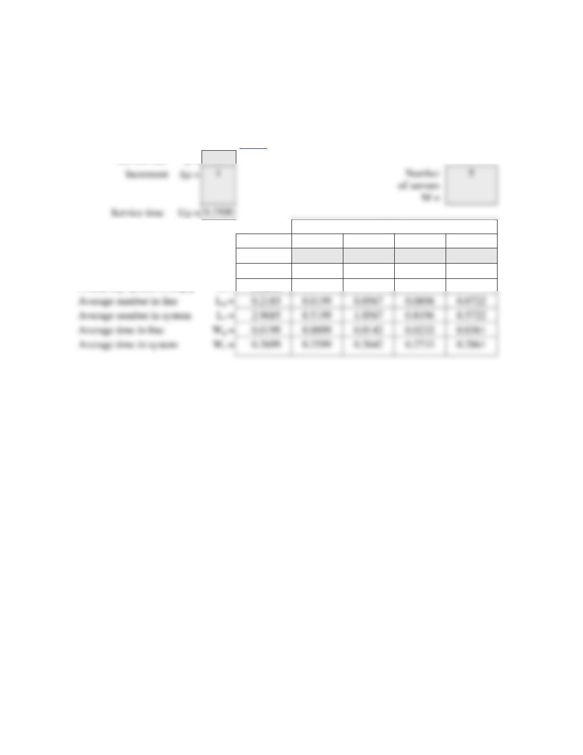
16.
Multiple Priorities Waiting Line Model
<Back
Service rate =
3
M =
Service time 1/ =
0.3333
Class
System
1
2
3
4
Arrival rate
=
11.0000
2
4
3
2
System Utilization
=
0.7333
Probability system is empty
P0 =
Average number in line
Average number in system
Ls =
Average time in system
M =
Service time 1/ =
0.2500
Chapter 18 – Management of Waiting Lines
18–12
16.
1 = 2/hr.
= 3/hr.
r =
=
11
= 3.7 [approx.]
a.
b.
A =
=
11
= .733
= 32.57
(1 – .733)1.265
From Table given above
W1 = .0333
W2 = 0.0555
W3 = .1202
W4 = .2705
c. Reducing the arrival rate of the second class to 3/hr. would increase the arrival rate of the
third class to 4/hr. The utilization would not change, nor would Lq or A change. B1 would not
change, so W1 and L1 would not be affected. Thus,
B1 = .87, W1 = .0333 hr., and L1 = (2)(.0333) = .0666
Using the following table we get the same results:
<Back
Service rate =
3
Increment =
1
Number
of servers
M =
5
Service time 1/ =
0.3333
Class
System
1
2
3
4
Arrival rate
=
11.0000
2
3
4
2
System Utilization
=
0.7333
Probability system is empty
Average number in line
Average number in system
Average time in line
M = 5 servers
From Table 18–4, Lq = 1.265
Chapter 18 – Management of Waiting Lines
18–13
d. The waiting time in any class is affected by the arrival rate for its class and the “B factor” of
the immediately higher priority class.
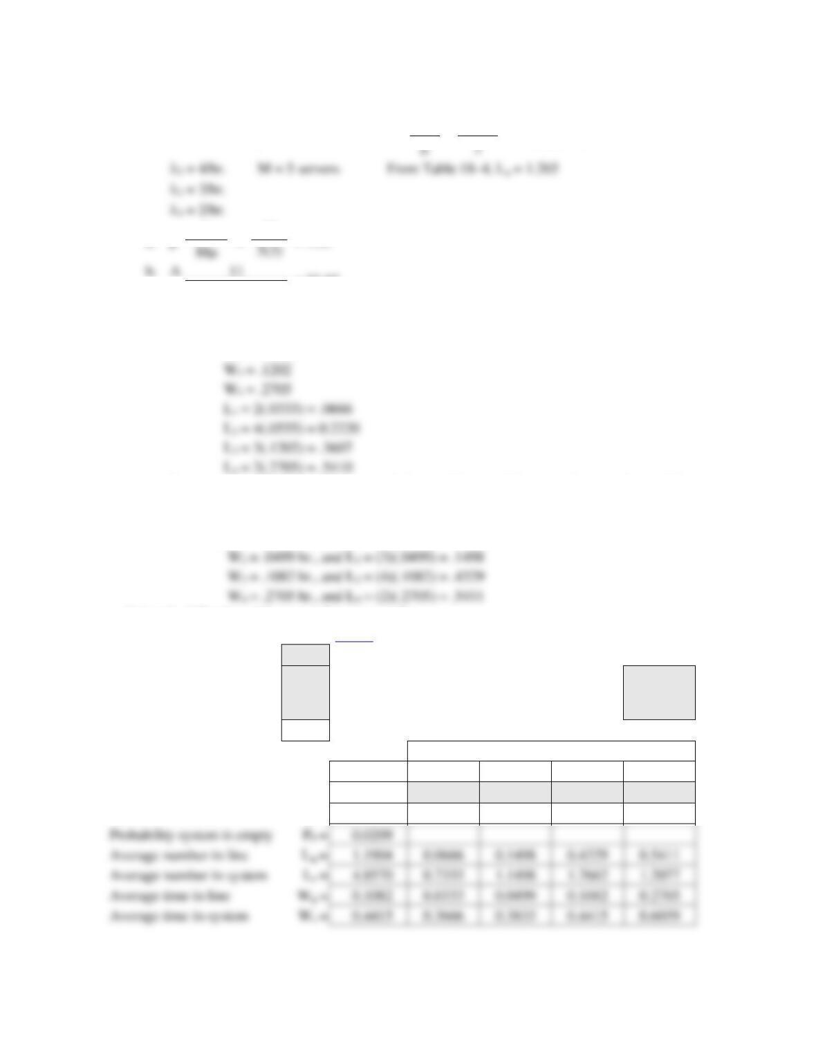
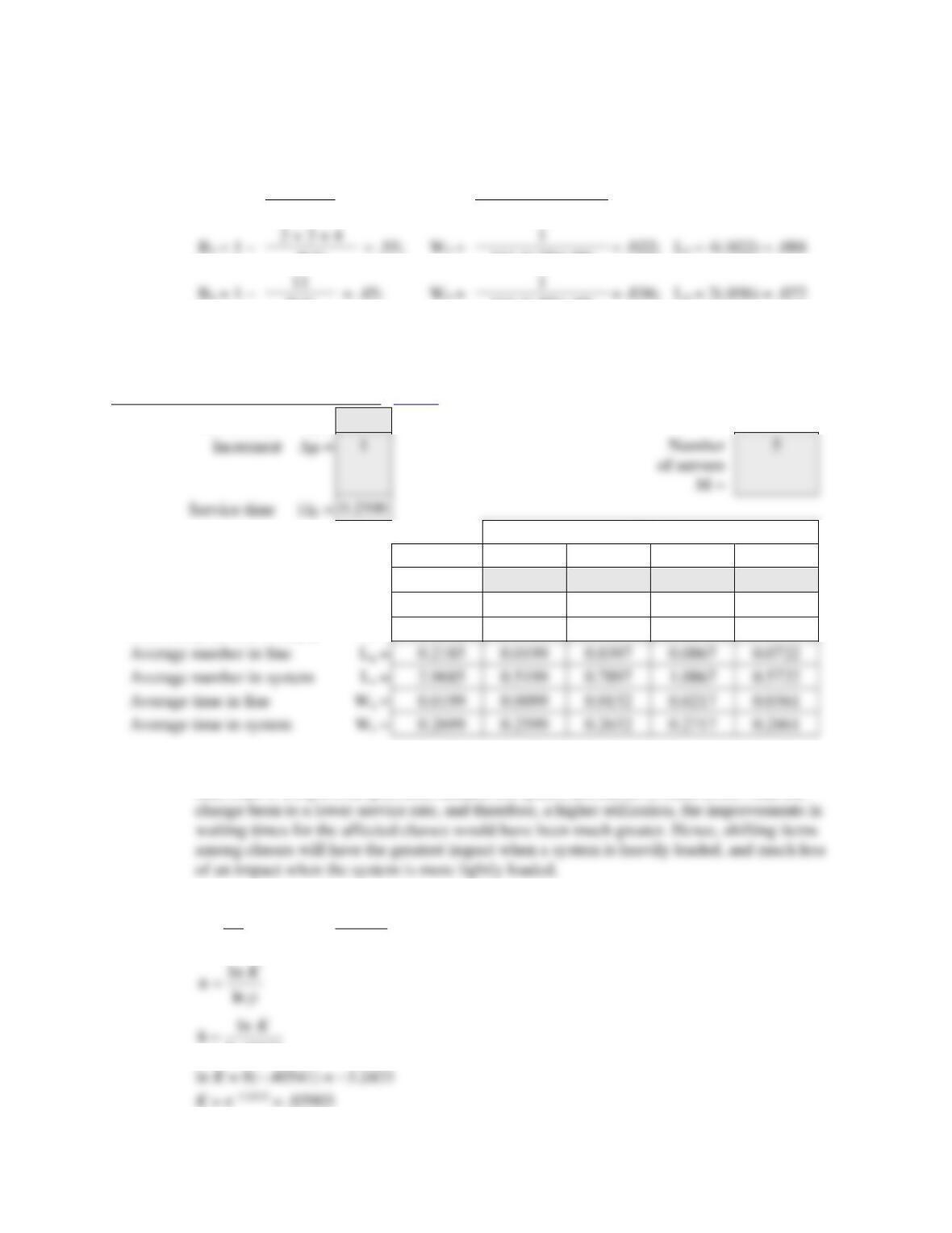
17. Using the following table we get the same results:
<Back
Service rate =
3
Class
System
1
2
3
4
Arrival rate
=
11.0000
2
4
3
2
System Utilization
=
0.5500
Probability system is empty
P0 =
0.0614
Average number in line
0.2185
Average time in line
0.0199
Chapter 18 – Management of Waiting Lines
18–14
Below are the numerical calculations for the Table provided above.
[Refer to #16 with = 4/hr. instead of 3/hr.]
11
5(4)
b.
= 111.1
Bo = 1
1
5(4)
111.1(1)(.90)
B2 = 1 –
= .70
W2 =
= .014
5(4)
111.1(.90)(.70)
B3 = 1 –
2 + 4 + 3
= .55
W3 =
1
= .023
5(4)
111.1(.70)(.55)
B4 = 1 –
2 + 4 + 3 + 2
= .45
W4 =
1
= .036
5(4)
111.1(.55)(.45)
L1 = 2(.010) = .020
L3 = 3(.023) = .069
L4 = 2(.036) = .072
r =
= 2.75 Lq = .22 [approx., interpolated.]
= .55
Chapter 18 – Management of Waiting Lines
18–15
c.
B1 = .90, W1 = .010, and L1 = .020
B2 = 1 –
2 + 3
= .75;
W2 =
1
= .013;
L2 = 3(.013) = .039
5(4)
111.1(.90)(.75)
5(4)
111.1(.75)(.55)
11
1
5(4)
111.1(.55)(.45)
Values in the above table are generated using the Excel templates from the DVD below
Multiple Priorities Waiting Line Model
<Back
Service rate =
4
Class
System
1
2
3
4
Arrival rate
=
11.0000
2
3
4
2
System Utilization
=
0.5500
Probability system is empty
P0 =
0.0614
Average number in line
0.2185
0.0199
0.0397
0.0867
0.0722
Average number in system
Average time in line
0.0199
0.0099
0.0132
0.0217
0.0361
Average time in system
0.2699
0.2599
0.2632
0.2717
0.2861
d. The improvement in waiting times for classes 2 and 3 is much less now (with a higher service
rate) than in the previous problem, because the system utilization is much lower. Had the
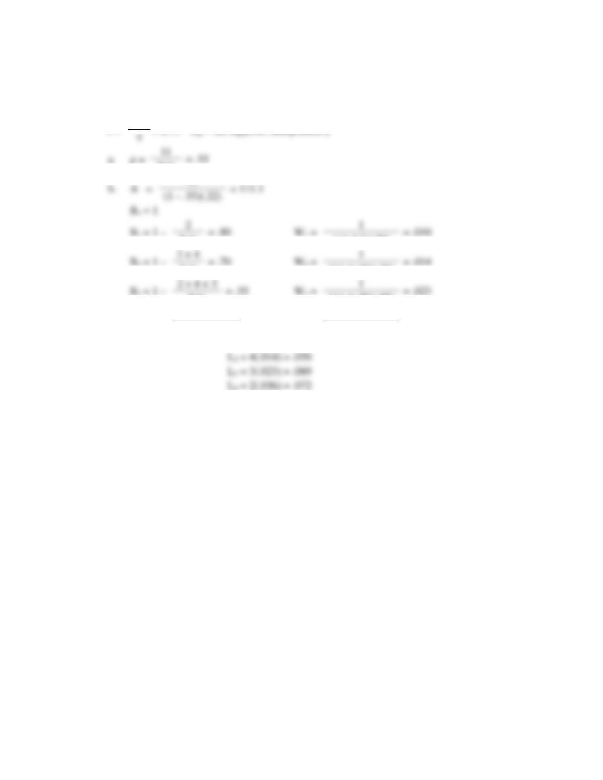
18. a.
6667.
)3)(20(
40
, 2
20
40
r====
6667.ln
B3 = 1 –
2 + 3 + 4
= .55;
W3 =
1
= .022;
L3 = 4(.022) = .088
Chapter 18 – Management of Waiting Lines
18–16
,
)1(L
Pr1
K
q−
−
=
solving for Pr
.03903 =
)66667.1)(889(.
Pr1
−
−
1− Pr = (.2963)(.03903) = .01156
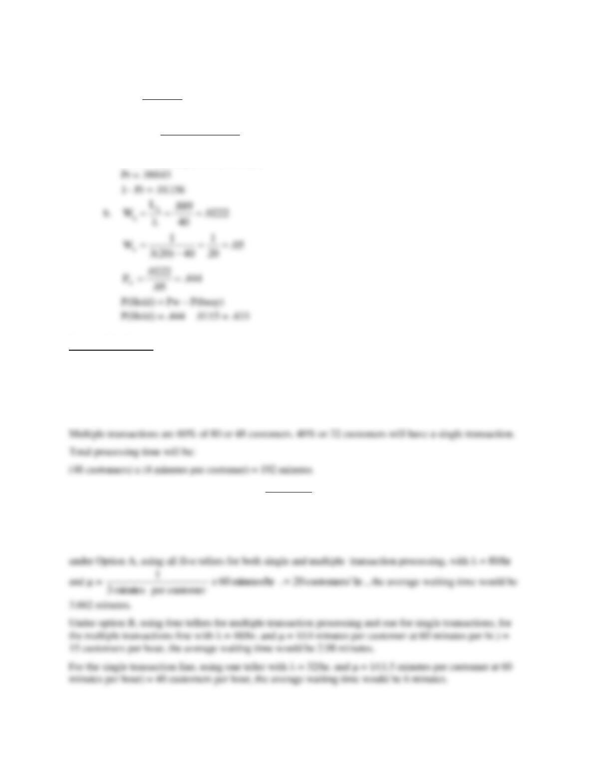
Case: Big Bank
Students must recognize that the arrival rate is 80 customers per hour, and that the separate teller would
constitute a single channel system. In order to determine times for the configuration in which the tellers
would handle both single and multiple transactions, students must first determine the average processing
time for that configuration.
Average processing time for Option A:
(32 customers) x (1.5minutes per customer) = 48 minutes
240 minutes
This means that for 80 customers, the average processing time would be:
240 minutes 80 customers = 3 minutes per customer
Chapter 18 – Management of Waiting Lines
18–17
Summary
Option Average waiting time in the line
A 1.66 minutes
The results indicate that the better choice would be to use a single line with five tellers processing both
single and multiple transactions. The disparity comes from the assumption (see the last assumption
below) that the idle tellers do not process customers from the “other” waiting line.
Assumptions:
a) The arrival rate is constant over the entire interval.